Week 16: 8 December
Tuesday and Friday
Monday
Week 15: 1 December
Wednesday and Thursday
Monday and Tuesday
Week 14: 24 November
Wednesday
Related Information:
Real and Imaginary parts of refractive index for water and ice as a function of wavelength (spreadsheet containing values).
MAX-DOAS: Using polarization in Multiple Angle Differential Optical Absorption Spectroscopy improves remote sensing of aerosols.
Tuesday
Monday
Week 13: 17 November
Thursday
Related Information:
Photograph of atmospheric haze due to the morning inversion and moist, cold morning.
Extreme coal burning air pollution in St. Louis, November 28th, 1939.
Wednesday
Related Information:
Circulations of warm and cool ocean water on the planet. Longer discussion at a introductory level.
Water vapor circulation during our last storm.
Tuesday
Monday
Week 12: 10 November
Thursday
Wednesday
Monday
Related Information:
Kelvin Helmholtz cloud from 11/6/2025.
Wave clouds.
Wave and diffraction simulator.
Week 11: 3 November
Thursday
Wednesday (Continue Chapter 3 Atmospheric Thermodynamics. Discuss HW5).
Tuesday (Continue Chapter 3 Atmospheric Thermodynamics. Discuss HW5).
Related Information:
Excellent introduction to radar.
Interpretation of satellite infrared imagery of the atmosphere and surface.
Current IR and Radar for the continental US (Product Overlays:Mesoanalysis:Composite Radar)
Monday (Continue Chapter 3 Atmospheric Thermodynamics. Discuss HW5).
Week 10: 27 October
Thursday (Continue Chapter 3 Atmospheric Thermodynamics. Discuss HW5).
Wednesday (Continue Chapter 3 Atmospheric Thermodynamics. Discuss HW5).
Tuesday (Continue Chapter 3 Atmospheric Thermodynamics. Discuss HW5).
Monday (Continue Chapter 3 Atmospheric Thermodynamics. Discuss HW5).
Week 9: 20 October
Thursday (Continue Chapter 3 Atmospheric Thermodynamics.)
Wednesday (Continue Chapter 3 Atmospheric Thermodynamics.)
Tuesday (Continue Chapter 3 Atmospheric Thermodynamics.)
Monday (Continue Chapter 3 Atmospheric Thermodynamics.)
Related Information:
Adiabatic process video to gain insight on air parcels (not saturated) undergoing expansion and compression without exchanging heat with the surroundings.
Derivation of equivalent potential temperature equation. And another that includes wet bulb potential temperature.
Week 8: 13 October
Monday Presentation on aerosol-cloud-radiation interactions and climate relevance in person at DMS106.
Tuesday-Thursday Zoom meetings while I'm on travel, not held in DMS106, but at your location of convenience.
Week 7: 6 October
Thursday (upcoming topics) (HW4 and HW5 coming up)
Look at the equation for saturation vapor pressure, model soundings, and the related information below.
Wednesday (upcoming topics) (HW4 and HW5 coming up)
Look at the equation for saturation vapor pressure, and the related information below.
Tuesday (upcoming topics) (HW4 and HW5 coming up)
Monday (upcoming topics) (HW4 and HW5 coming up)
Related Information:
Photographing snowflakes with your cell-phone.
Saturation vapor pressure calculator online.
DESI has lightning forecasts under Convection and Precipitation forecasts, and model soundings.
To create a recent model sounding using HRRR as was presented in class on Thursday Oct. 3, start at the Continental US scale and click on any point. This will bring up a sounding. Choose on where radar indicates active precipitation, and compare with another elsewhere. Notice the Dendrite Grow Zone (DGR) elevations and associated temperatures.
Week 6: 29 September
Tuesday, Wednesday, and Thursday
To create a recent model sounding using HRRR as was presented in class on Thursday Oct. 3, start at the Continental US scale and click on any point. This will bring up a sounding. Choose on where radar indicates active precipitation, and compare with another elsewhere. Notice the Dendrite Grow Zone (DGR) elevations and associated temperatures.
Monday
Related Information:
Model soundings from DESI (Dynamic Ensemble Scenarios for Impact-Based Decision Support).
Week 5: 22 September
Thursday
After having read chapter 1, read chapter 3:
In preparation, install Microsoft Office (including Excel) on your laptop if needed (use your netID to login to Office 365 and find the installation link for Office).
We will also use Google Earth, available here for use on the web, or here to install in your laptop.
Tuesday and Wednesday
After having read chapter 1, read chapter 3.
Continue with HW3 parts c-g.
It involves working with sounding data, both with calculations and graphs.
Students are encouraged to bring their laptop or use the computers in the classroom.
If using classroom computers be sure to save your work in your cloud or USB drive because everything is erased when logging out of the classroom computers.
In preparation, install Microsoft Office (including Excel) on your laptop if needed (use your netID to login to Office 365 and find the installation link for Office).
We will also use Google Earth, available here for use on the web, or here to install in your laptop.
Monday
Begin HW3. It will involve working with sounding data, both with calculations and graphs. We will go through much of it in class.
Students can bring their laptop or use the computers in the classroom.
If using classroom computers be sure to save your work in your cloud or USB drive because everything is erased when logging out of the classroom computers.
I will use Excel, though you are welcome to follow along and to use Python or other software.
In preparation, install Microsoft Office (including Excel) on your laptop if needed (use your netID to login to Office 365 and find the installation link for Office).
We will also use Google Earth, available here for use on the web, or here to install in your laptop.
Week 4: 15 September
Thursday
Outcome:
We discussed the Reno soundings. OneNotes from the day as a PDF.
Plan:
Discuss Reno morning and afternoon sounding examples for recent days
(12Z and 0z) from the Univ. of Wyoming site. OneNote.
Begin HW3. It will involve working with sounding data, both with calculations and graphs. We will go through much of it in class.
Students can bring their laptop or use the computers in the classroom.
If using classroom computers be sure to save your work in your cloud or USB drive because everything is erased when logging out of the classroom computers.
I will use Excel, though you are welcome to follow along and to use Python or other software.
In preparation, install Microsoft Office (including Excel) on your laptop if needed (use your netID to login to Office 365 and find the installation link for Office).
We will also use Google Earth, available here for use on the web, or here to install in your laptop.
Wednesday
Discuss Goal 2. Then finish discussion of lapse rate in Goal 1.
All of the Online HW has been posted in WebCampus for the rest of the semester. They may be useful for projects. Due dates are a guideline for when we'll be covering the subjects.
Plan:
Goal 1: Further the understanding of SkewT diagrams
Lapse rate discussion, continued PPT.
Reno morning and afternoon sounding examples for recent days
(0Z and 12Z) from the Univ. of Wyoming site. OneNote.
Goal 2: Homework 2: Continue with SkewT development, Lapse Rate.
Discuss HW2 problem by problem. Problem 1. Supply reference(s) used, including AI.
Problem 2.
Define lapse rate as a derivative and as a finite difference. See the lapse rate discussion. Go to the south pole station and view sounding text and GIF skewTs. OneNote.
Python script for retrieving soundings from the Univ. Wyo radiosonde data server, calculating the lapse rate, finding the minimum lapse rate, and graphing the lapse rate as a function of time.
Tuesday
Complete Goal 3. Then Goal 2. Then finish discussion of lapse rate in Goal 1.
All of the Online HW has been posted in WebCampus for the rest of the semester. They may be useful for projects. Due dates are a guideline for when we'll be covering the subjects.
Plan:
Goal 1: Further the understanding of SkewT diagrams
Lapse rate discussion, continued PPT.
Reno morning and afternoon sounding examples for recent days
(0Z and 12Z) from the Univ. of Wyoming site. OneNote.
Goal 2: Homework 2: Continue with SkewT development, Lapse Rate.
Discuss HW2 problem by problem. Problem 1. Supply reference(s) used, including AI.
Problem 2.
Define lapse rate as a derivative and as a finite difference. See the lapse rate discussion. Go to the south pole station and view sounding text and GIF skewTs. OneNote.
Python script for retrieving soundings from the Univ. Wyo radiosonde data server, calculating the lapse rate, finding the minimum lapse rate, and graphing as a function of time.
Goal 3: HW2 Introduce large scale circulation of the atmosphere:
Example problem on atmospheric mass carried by trade winds.
Homework problem on annual hemispherically averaged pressure oscillation.
Problem 3.
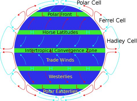
Discuss tradewinds and global circulation in general, and for problems 1.20 and 1.21 starting with slide 45 of Chapter 1 presentation.
Discuss problem 1.21 for HW2. OneNote.
Image showing the idealized average global circulation (source).
Monday
Plan:
Goal 1: Further the understanding of SkewT diagrams
Lapse rate discussion, continued PPT.
Reno morning and afternoon sounding examples for recent days
(0Z and 12Z) from the Univ. of Wyoming site. OneNote.
Goal 2: Homework 2: Continue with SkewT development, Lapse Rate.
Discuss HW2 problem by problem. Problem 1. Supply reference(s) used, including AI.
Problem 2.
Define lapse rate as a derivative and as a finite difference. See the lapse rate discussion. Go to the south pole station and view sounding text and GIF skewTs. OneNote.
Goal 3: HW2 Introduce large scale circulation of the atmosphere:
Example problem on atmospheric mass carried by trade winds. Homework problem on annual hemispherically averaged pressure oscillation.
Problem 3.
Discuss tradewinds and global circulation in general, and for problems 1.20 and 1.21 starting with slide 45 of Chapter 1 presentation.
Discuss problem 1.21 for HW2. OneNote.
Model for average global circulation (source).
Related Information:
Turbulence and vortex rings in air video to visualize the air motions likely happening in the planetary boundary layer and get an introduction to turbulence.
Adiabatic process video to gain insight on air parcels (not saturated) undergoing expansion and compression without exchanging heat with the surroundings.
Week 3: 8 September
Thursday
Outcome: Reviewed stability; discussed sub and super adiabatic examples; inversions and link to net upwelling infrared radiation in the atmosphere along with a calculation to quantify if from UNR weather station data; neutral stability, potential temperature equation meaning and use in a graph to represent stability; and development of the planetary boundary layer during the day, not necessarily in that order. Notes were made in the PPT that will be posted when we are finished with these sections.
Plan:
Goal 1: Further the understanding of SkewT diagrams https://www.youtube.com/watch?v=_UoTTq651dE
Lapse rate discussion, continued PPT.
Reno morning and afternoon sounding examples for recent days
(0Z and 12Z) from the Univ. of Wyoming site. OneNote.
Goal 2: Homework 2: Continue with SkewT development, Lapse Rate.
Discuss HW2 problem by problem. Problem 1. Supply reference(s) used, including AI.
Problem 2.
Define lapse rate as a derivative and as a finite difference. See the lapse rate discussion. Go to the south pole station and view sounding text and GIF skewTs. OneNote.
Goal 3: HW2 Introduce large scale circulation of the atmosphere:
Example problem on atmospheric mass carried by trade winds. Homework problem on annual hemispherically averaged pressure oscillation.
Problem 3.
Discuss tradewinds and global circulation in general, and for problems 1.20 and 1.21 starting with slide 45 of Chapter 1 presentation.
Discuss problem 1.21 for HW2. OneNote.
Wednesday
Plan:
Goal 1: Further the understanding of SkewT diagrams
Lapse rate discussion. PPT.
Reno morning and afternoon sounding examples for recent days
(0Z and 12Z) from the Univ. of Wyoming site. OneNote.
Goal 2: Homework 2: Continue with SkewT development, Lapse Rate.
Discuss HW2 problem by problem. Problem 1. Supply reference(s) used, including AI.
Problem 2.
Define lapse rate as a derivative and as a finite difference. Go to the south pole station and view sounding text and GIF skewTs. OneNote.
Goal 3: HW2 Introduce large scale circulation of the atmosphere:
Example problem on atmospheric mass carried by trade winds. Homework problem on annual hemispherically averaged pressure oscillation.
Problem 3.
Discuss tradewinds and global circulation in general, and for problems 1.20 and 1.21 starting with slide 45 of Chapter 1 presentation.
Discuss problem 1.21 for HW2. OneNote.
Tuesday
Outcome: Links are to OneNote pages. This program is part of Microsoft Office. Use your NetID to login to Office 365 and you can download Microsoft Office to your computer. It can also be used online.
To view in OneNote, right click on the link and save it to your computer (or iPad).
You can create a section and put all of your pages in one section.
OneNotes on precipitable water and introduction to atmospheric rivers.
OneNotes on more discussion of atmospheric rivers and related meteorology.
OneNotes on comparison of Reno and Slidell SkewT diagrams.
Plan:
Goal 1: Further the understanding of SkewT diagrams
Additional discussion of Atmospheric Rivers (ARs) and the meteorology associated with them.
Review HW1: Reno and Slidell LA soundings main features. OneNote.
Reno morning and afternoon sounding examples for recent days
(0Z and 12Z) from the Univ. of Wyoming site. OneNote.
Goal 2: Homework 2: Continue with SkewT development, Lapse Rate.
Discuss HW2 problem by problem. Problem 1. Supply reference(s) used, including AI.
Problem 2.
Define lapse rate as a derivative and as a finite difference. Go to the south pole station and view sounding text and GIF skewTs. OneNote.
Goal 3: HW2 Introduce large scale circulation of the atmosphere:
Example problem on atmospheric mass carried by trade winds. Homework problem on annual hemispherically averaged pressure oscillation.
Problem 3.
Discuss tradewinds and global circulation in general, and for problems 1.20 and 1.21 starting with slide 45 of Chapter 1 presentation.
Discuss problem 1.21 for HW2. OneNote.
Monday
Outcome:
Discussed wind barbs, wind direction and speed, and meteorological wind angle.
Discussed precipitable water, equation to calculate it, typical values, and example of water vapor transport in an Atmospheric River event.
Plan:
Goal 1: Further the understanding of SkewT diagrams
Discuss wind barbs ane meteorological wind direction. (OneNote).
Define and discuss Precipitable Water Vapor (PWV). Atmosperic river example. OneNote.
Review HW1: Reno and Slidell LA soundings main features. OneNote.
Reno morning and afternoon sounding examples for recent days
(0Z and 12Z) from the Univ. of Wyoming site. OneNote.
Goal 2: Homework 2: Continue with SkewT development, Lapse Rate.
Discuss HW2 problem by problem. Problem 1. Supply reference(s) used, including AI.
Problem 2.
Define lapse rate as a derivative and as a finite difference. Go to the south pole station and view sounding text and GIF skewTs. OneNote.
Goal 3: HW2 Introduce large scale circulation of the atmosphere:
Example problem on atmospheric mass carried by trade winds. Homework problem on annual hemispherically averaged pressure oscillation.
Problem 3.
Discuss tradewinds and global circulation in general, and for problems 1.20 and 1.21 starting with slide 45 of Chapter 1 presentation.
Discuss problem 1.21 for HW2. OneNote
Related Information:
Turbulence and vortex rings in air video to visualize the air motions happening in the planetary boundary layer.
Fire breaks out (GOES imagery) suddenly on the west side of the Sierra Nevada Mountains. Pyrocumulus and lee wave clouds can be seen.
Blank skewT with definitions.
Wind barbs.
Hot air balloons are an example of buoyancy introduced by lowering density by increasing temperature.
|
Week 2: 1 September
Thursday
Plan:
Discuss relative humidity calculation for the Wednesday sounding, at the surface and near the LCL.
Find the wetbulb and wetbulb potential temperature values.
Discuss the steps for obtaining each value we've discussed so far.
Look at times Reno soundings for the last few days (0Z and 12Z).
Blank skewT with definitions.
Wind barbs.
Look at an example skewT diagram from the Univ. of Wyoming site.
Related Information:
|
Wednesday
Outcome:
Discussed the use of a logarithmic scale for pressure to be used along with altitude for height, and then the skewed temperature axis for isotherms.
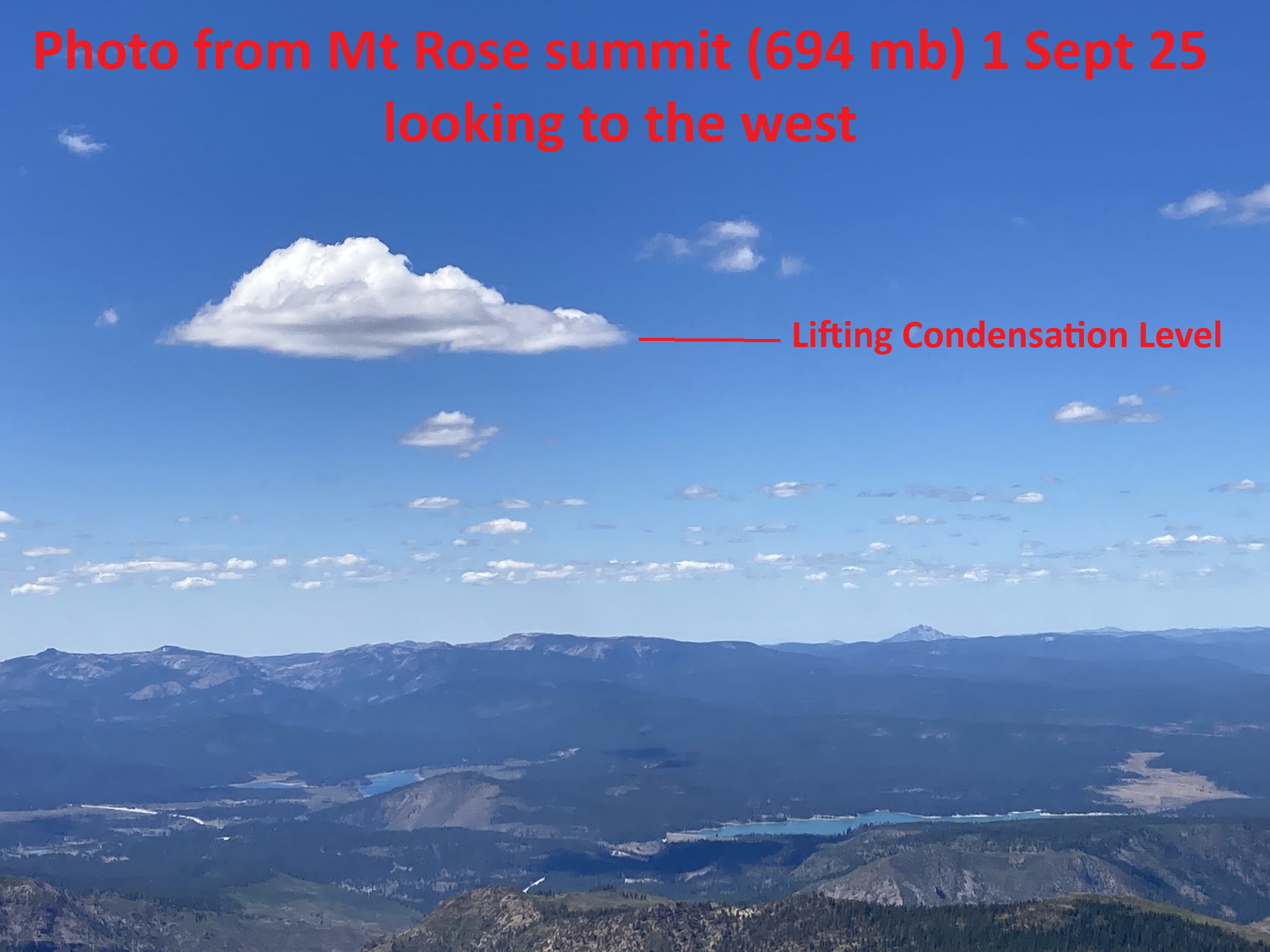
Chose room temperature and dewpoint conditions along with a surface pressure of 694 mb to find the LCL, introducing the lines of constant mixing ratio,
dry adiabats, potential temperature, and moist adiabats to raise air parcels above the LCL.
Plan:
Continue discussing skewT-logP thermodynamic diagrams.
We will return to this topic often during the semester to add understanding.
Homework 1 is an introduction to these diagrams.
Blank skewT with definitions.
Wind barbs.
Look at an example skewT diagram from the Univ. of Wyoming site.
Tuesday
Outcome:
Discussed mirages and the use of Snell's law and the variation of air density with height to understand them. Started discussion of skewT-logP graphs.
Plan:
Density variation with height: Autoconvecting atmosphere and relation to mirages using density being linearly proportional to refractive index and Snell's law.
Pressure measurement with a mercury barometer and modern barometer. (OneNote document: Right click and save the document. Then open it with OneNote).
Discuss skewT-logP Thermodynamic diagrams.
Blank skewT with definitions.
Wind barbs.
Look at an example skewT diagram from the Univ. of Wyoming site.
Related Information:
Integrated Global Radiosonde Archive (IGRA) from NOAA.
Data availability from IGRA.
Video describing locations to obtain radiosonde data.
Reno Weather Data
Simplified Reno example soundings with a simplified skewT-logP diagram for the end of August and early September 2024.
Single sounding. Overlay of a still morning and afternoon sounding, and another example with well-mixed windy day.
UNR weather station data for pressure and windspeed.
Soundings for windy Monday afternoon and calm Tuesday morning (0z and 12z soundings on 9/3/2024) including water vapor mixing ratio curves.
Reno 9/3/24 afternoon and 9/4/24 morning soundings overlaid with the LCL, dry adiabats, and mixing ratio lines.
Reno 9/3/24 afternoon sounding with lifted air parcel, LCL, dry and moist adiabats, and mixng ratio lines.
Reno soundings for:
Rainy day
Dry day
Program for overlaying two soundings.
Week 1: 25 August
Thursday
Outcome: Discussed pressure, and density in the atmosphere and underwater, for compressible and nearly incompressible fluids (air and water).
Plan: Note: Zoom is being used for a student that can't come to class in person. Class will be held as usual in DMS106.
Discuss pressure, and density in the atmosphere and underwater.
Density and ray optics example, mirages.
Pressure as a scalar field associated with momentum transport.
Discuss skewT-logP Thermodynamic diagrams.
Blank skewT with definitions.
Wind barbs.
Look at an example skewT diagram from the Univ. of Wyoming site.
Related Information:
Approximate theory for spectral clear sky downwelling IR.
Wednesday
Outcome:Discussed reason for nitrogen molecule being most dominant in the Earth's atmosphere.
Talked about vibrational and rotational modes of infrared active gases and how to calculate infrared emissivity for gas layers.
Began discussion of pressure, definition, units, and started example of travel over Donner summit to San Francisco.
Plan: Atmospheric composition discussion (Presentation).
Discuss pressure, density and examples, mirage.
Pressure as a scalar field, momentum transport.
Pressure underwater.
Pressure measurement with a mercury barometer and modern barometer. (OneNote document: Right click and save the document. Then open it with OneNote).
Related Information:
Pressure definitions, how they are used. Reduction of station pressure to sea level value for comparing weather conditions at different altitudes.
Atmospheric electricity discussion and simplified measurement method demonstration.
Fair weather electric field discussion and demonstration.
Construction and use of electric field mill instrument, and another version.
Tuesday
Plan: Continue Atmospheric Physics general discussion and atmospheric composition (Presentation).
Discuss pressure, density and examples, mirage.
Pressure definitions, how they are used. Reduction of station pressure to sea level value for comparing weather conditions at different altitudes.
Related Information:
NOAA's environmental webinar series covering a wide range of topics. Some are available from archives. You can sign up for email notifications.
Monday
Outcome: Student introductions, syllabus, homework discussion, and started discussion of Atmospheric Physics. Thanks for the questions 😀
| Introductions -- each student introduce themselves. |
| Syllabus. |
| Homework. |
| Webcampus for online homework assignments/reading. |
|
Online Homework 1 is due 31 August. See webcampus. This is based on MetEd. Intro to the Atmosphere. Online Homework 2 is due 7 September. See webcampus. This is based on MetEd. Meteorological charting. Homework 1 is due 5 September, to be turned in through web campus. For this week: Read chapter 1. |
The final project has been posted. |
This class includes:
Lecture/discussion in class.
Active class participation/activity involving atmospheric data from around the world.
Study using online modules for atmospheric science education.
Chapter 1: Introduction and overview:
Overview Presentation: Atmospheric Science relies heavily on measurements and models!
Composition of the Earth's atmosphere.
Next discuss atmospheric pressure and density (OneNote).
Mass of the atmosphere calculation using an online Python editor and this AI query1 for code generation.
Vertical structure of the atmosphere image.
Related Information:
Perhaps useful items.