ATMS 360 Homework and Course Deliverables (return to main page)
[How to write lab report]
Assignment 10:
Lee wave clouds in the atmosphere downwind of the Sierra Nevada mountain range:
Study using balloon-sounding atmospheric data and satellite observations.
Turn in this homework assignment through webCampus, prepared using Powerpoint.
Presentations will follow.
Observation of lee wave clouds in the atmosphere and potential problems with radiosonde measurements of atmospheric temperature due to sensor wetting.
EXAMPLES OF LEE WAVE CLOUDS
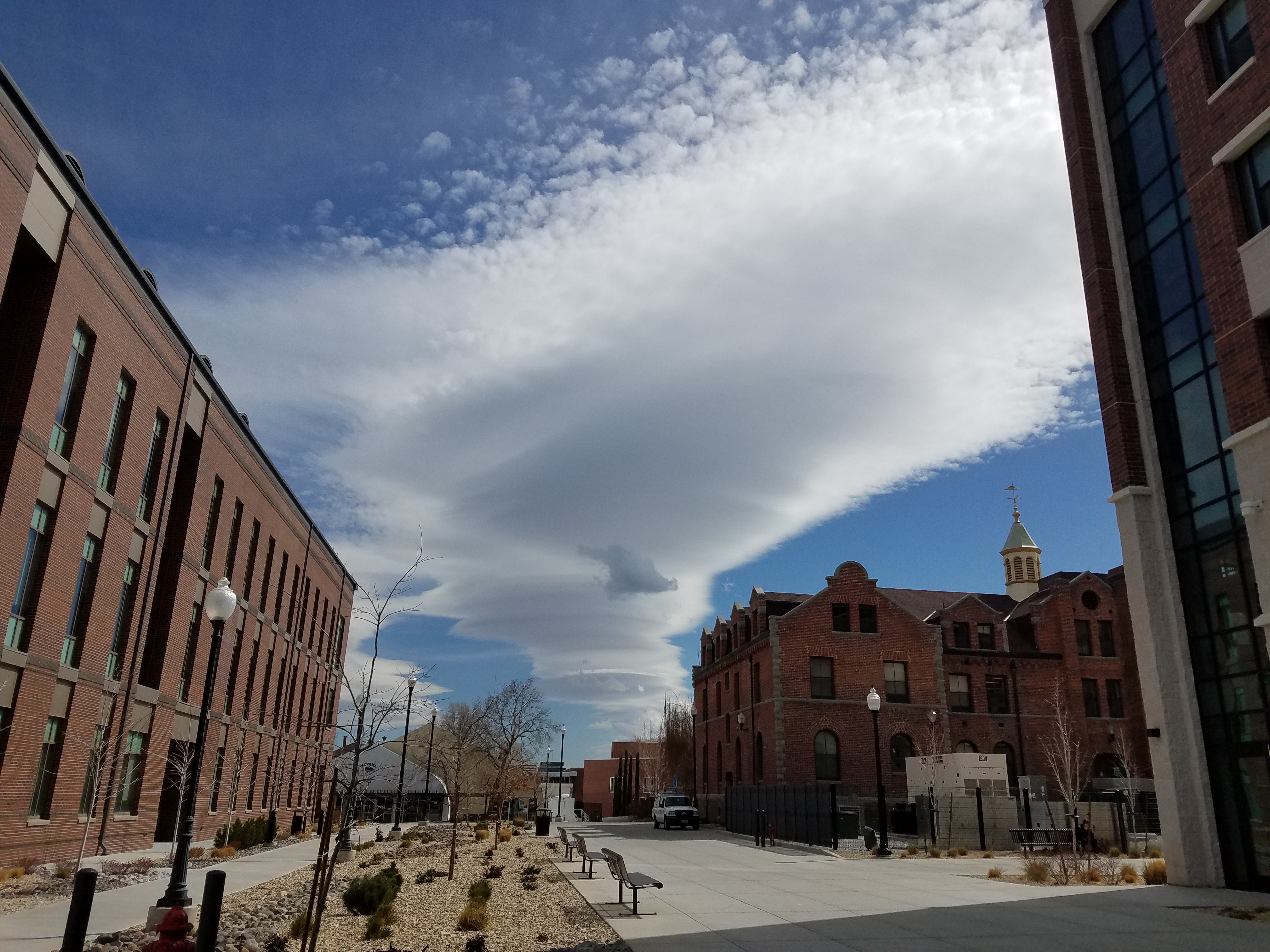
Photograph of a wavecloud from the top of the Physics building at UNR on the 7th of April 2021 at around 4 pm local time.
Photograph by Ally of the same cloud earlier in the day.
Here is a close-up animation from Jonathan for a day in the life of lee wave clouds to give an idea of the type of clouds we're looking for.
The larger area animation shows the origin of the long wavelength wave that collides with the the lee waves to disrupt them for awhile.
Lee wave clouds and others in Reno.
ADDITIONAL RESOURCES AND ASSIGNMENTS FOR LATER:
Rough draft of notes with questions, and derivation of trapped lee waves. (Gemini).
Use the IR single image near the time of the wavecloud to get cloud top temperature and ground temperature and compare with sounding.
Calculate lapse rate from sounding and compare with value obtained from wave cloud wavelength.
Put the NASA AQUA image into google earth and overlay with the sounding KML file generated from webpage below. Only works for specific years when the raw file format was updated. (most recent). Convenient that the Aqua overpass is getting later, closer to balloon launch time. Measure wavelength using Aqua image and directly getting wavelength from the ruler tool in Worldview.
Use reanalysis to get the 700 mb and 500 mb level meteorology to explain mechanism of flow. use wide enough area to make it clearly visible.
Purpose:
1. Learn about radiosonde measurements (balloon-soundings of the atmosphere), satellite imagery, and an important cloud type for us in Reno, lee wave clouds, also known as gravity wave clouds.
2. Help diagnose issues with radiosondes when they exit clouds after wetting the temperature sensor. Evaporative cooling of cloud water from the sensor gives abnormally low temperatures until the water evaporates completely.
Deliverable: A Powerpoint presentation with topics and slides as follows. Each Topic can be 1 slide, or more if needed.
Each student needs to choose a unique day and lee wave cloud observation for their study by using NASA AQUA MODIS satellite imagery and/or GOES geostationary satellite imagery.
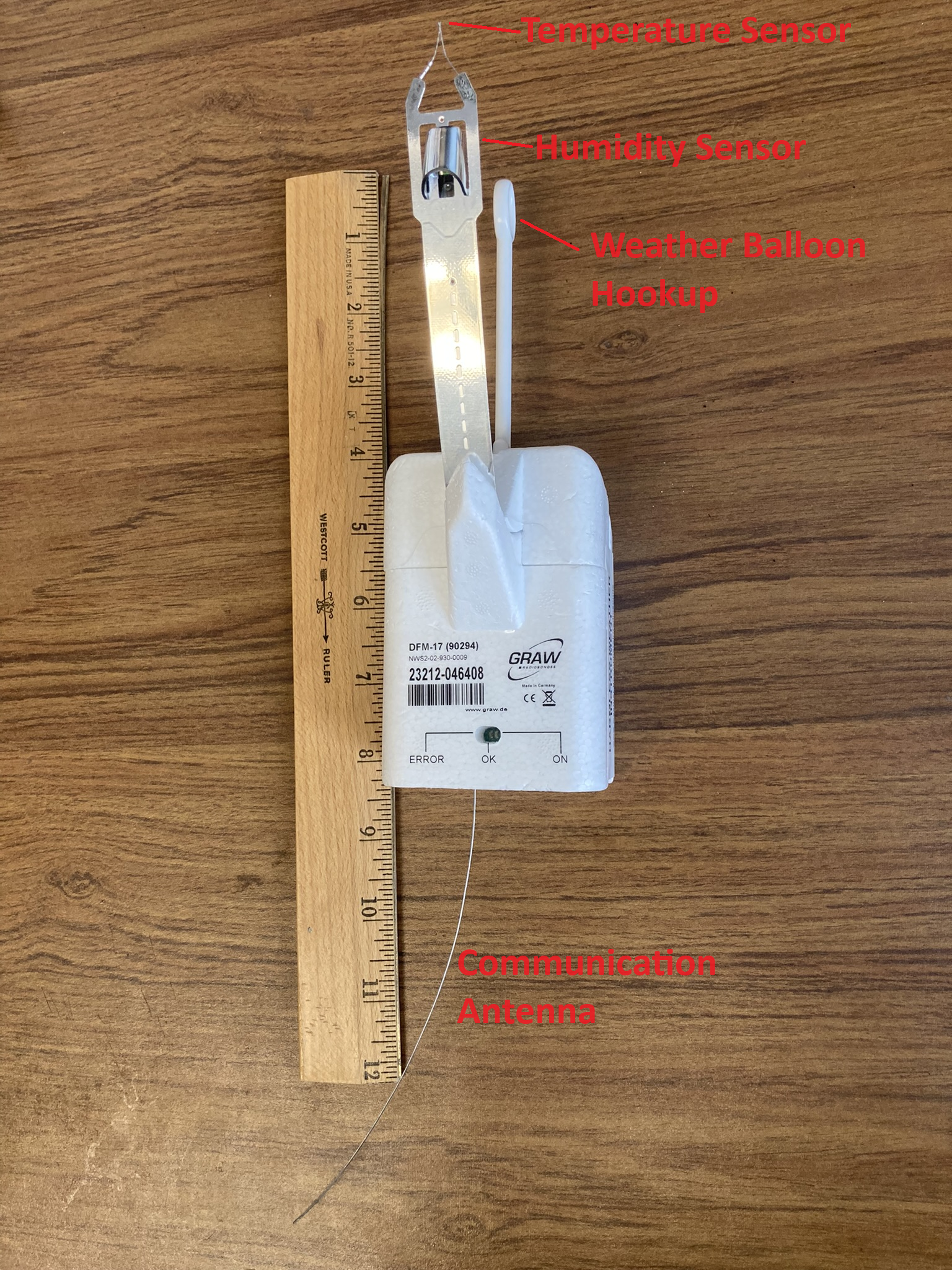
Topic 1 (same for everyone): Briefly describe radiosonde observations of the atmosphere in general.
Here is the type of radiosonde in use at the Reno and other National Weather Service (NWS) offices.
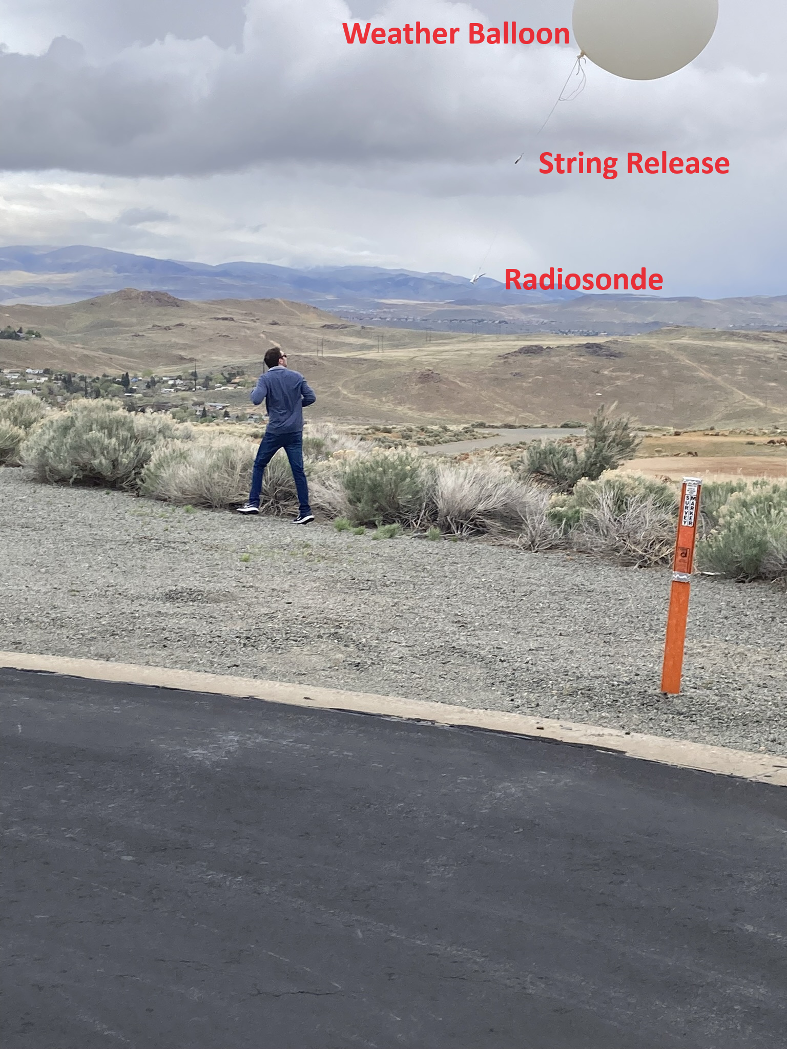
Weather balloon launch (picture) from the Reno NWS office on 4/26/2024.
Brochure describing the radiosonde currently in use at the Reno NWS.
Topic 2 (same for everyone): Define air temperature, dewpoint temperature, and wetbulb temperature.
Discuss
what happens to radiosonde when the temperature sensor is wetted due to passage through and cloud and then enters drier conditions above.
We will do lab measurements of each temperature using an IR camera and IR temperature sensors.
Cotton pads are used to measure air temperature and, after wetting the pad, wet bulb temperature. Use wires with alligator clips to rotate the wet pad and ventilate it well before measurement.
Take a cold microscope slide from the freezer. Frost or dew will begin to form on it. Just as the frost or dew begins to dissipate, record its temperature as the dewpoint (or frost point) temperature.
Read pressure from the Teensy 3.2 balloon sounding card using a Freescale pressure transducer, Sensirion SHT75 T and RH sensor, and the enclosed sketch.
Use Normand's rule to find the lifting condensation level and to check the three temperature measurements for consistency.
Images. Teensy sketches for reference (not needed for presentation).
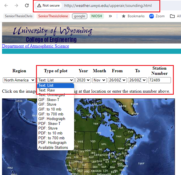
Topic 3: Obtain the atmospheric skewT-logP GIF image sounding for the time and date of your case study, of air, dewpoint temperature and winds.
Here's where to get data: Standard resolution radiosonde data: High resolution radiosonde data.
We will discuss these diagrams.
Here is an introduction.
Use Powerpoint, Paint or other graphics program to highlight the 0 degree and -40 degree isotherms.
The ridge line for the Sierras near Reno is at about 700 mb. Highlight the 700 mb isobar.
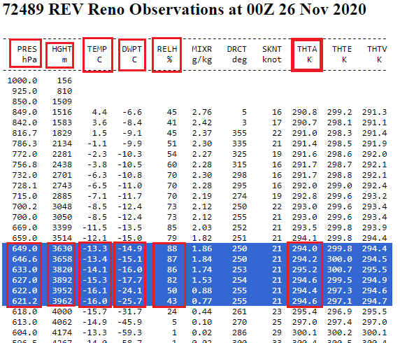
NOTE: The 26 Nov 2020 at 0z sounding is the one relevant for the 25 November 2020 MODIS image for the example wavecloud in Topic 6.
This sounding is in the afternoon, approximately 4.5 hours after the satellite image.
Here's an example of a marked up skewT-logP sounding with details to also label parts of the diagram.
Clouds are likely to form when the dewpoint temperature is very close to the air temperature.
Circle the likely layer, probably in the range 500-700 mb level, that is associated with the wavecloud, if there is one.
Topic 4: Screen shot of the atmospheric sounding data that highlights the data near where the likely level of the wavecloud is located (here's how to get it).
(Here's where to get data: Standard resolution radiosonde data: High resolution radiosonde data).
Here's a marked up example.
For the example wave cloud, the layer from 649 mb to 621.2 mb is likely the one for the cloud and the start of the drier layer above it.
Note especially a possible circumstance where the RELH (relative humidity) is above 80% or so, and if THTA (potential temperature) decreases with height in that same layer.
The RELH (relative humidity) ranges 88% to 43% in that layer.
The reduction of THTA and with increasing height in that layer is likely due to evaporative cooling of the temperature sensor that got covered with water passing through a cloud, that then evaporated and cooled the sensor as it entered the dry layer above. It is likely that the atmospheric layer would be falsely interpreted as being unstable. Note that not all soundings will have a layer like the one described here, and it's possible that the wavecloud dissipated in the time between when the satellite image was obtained and when the sounding was obtained.
EXTRA CREDIT: Excel sheet example for calculating the lapse rate from the lee wave cloud wavelength, and other sounding information. It compares this with the observed lapse rate, also calculated with the spreadsheet. Obtain the cloud top radiance and convert it to the wave cloud top temperature using the Channel 13 clean IR imagery.
Hover over a single loaded image using WCT and note the radiance value.
Use this temperature and your sounding to obtain the cloud top pressure.
This helps identity the layer of the atmosphere responsible for the lee wave cloud.
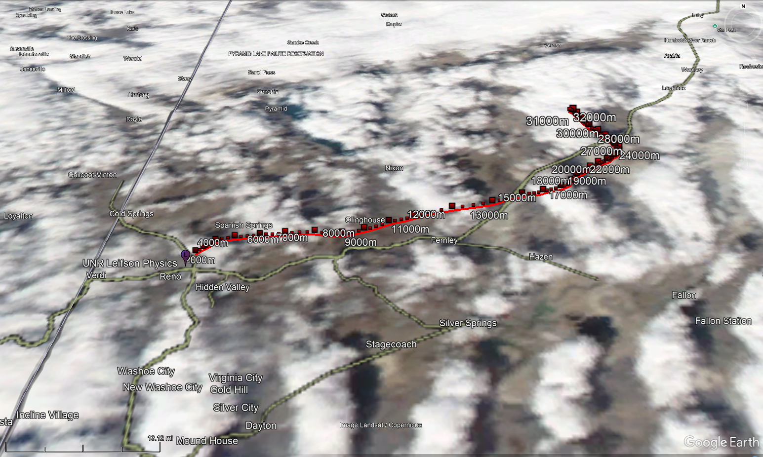
To investigate further, save the satellite image from Aqua MODIS Worldview at a KMZ file. Read it into Google Earth.
Use this script to obtain a balloon trajectory file in KML format for input Google Earth.
Here's an example.
Topic 5 (same for everyone): Briefly show and discuss how polar orbiting satellite imagery is obtained from the NASA AQUA satellite, equipped with Moderate Resolution Imaging Spectrometers (MODIS) instrument used to image clouds. This video shows how the MODIS instrument on AQUA acquires images of the atmosphere (from here).
The AQUA satellite overpass was at approximately 1:30 pm local standard time in Reno, though it has been getting later as the satellite ages.
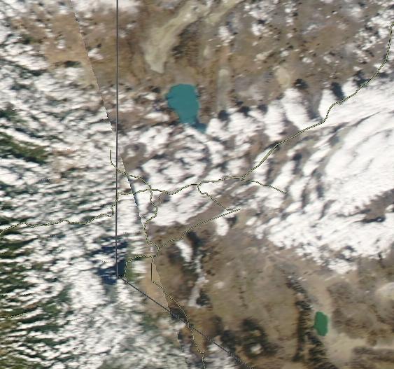
Topic 6: Obtain a NASA MODIS/AQUA satellite image showing lee wave clouds downwind of the Sierra Nevada Mountains for a specific day of your choosing.
Add this image to your presentation (screen shot or snapshot).
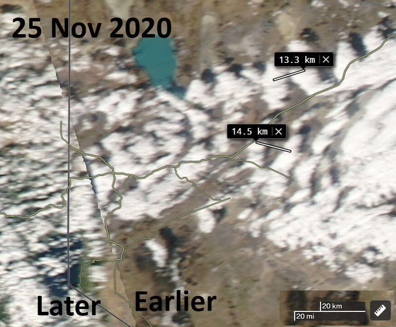
Example image from 25 November 2020 at 20z. (local backup). Here's how to find the time of the AQUA satellite overpass within NASA Worldview.
Topic 7: Use the measuring tool to measure the wavelength at several points. Take a screen shot and include it in your presentation (example).
Extra: Calculate the wavelength from the lapse rate, wind speed, and temperature (Theory) (or calculate lapse rate from the other information).
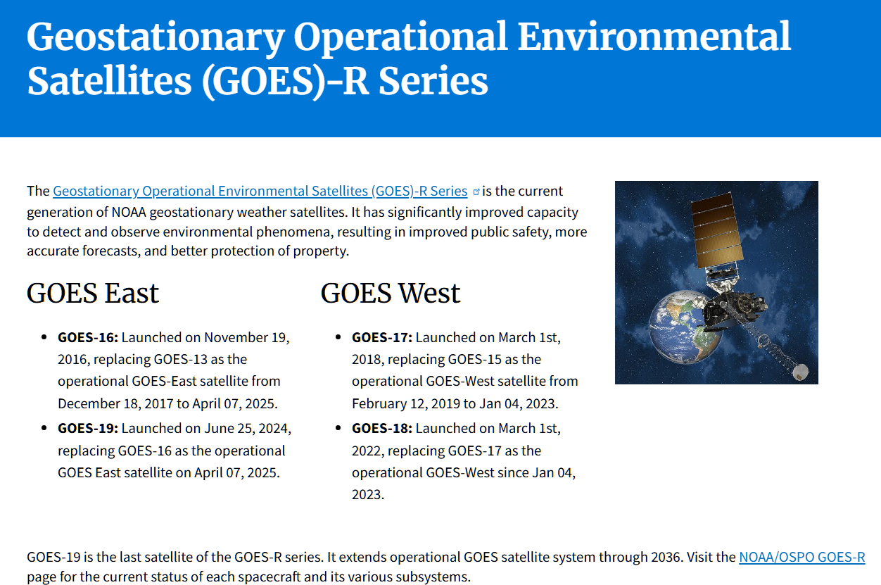
Topic 8: Look at the cloud under solar illumination during daylight hours by making an animation for your presentation using the Geostationary Operation Environmental Satellite (GOES) data obtained using the NOAA Weather and Climate Toolkit. Use channel 1 visible wavelength data. Instructions. Here is a summary of the recent and current GOES satellites.
Topic 9: Show the evolution of the cloud by obtaining an IR channel observation using GOES data obtained with the NOAA Weather and Climate Toolkit. Use channel 13 clean-IR data. Instructions.
Load the last from (time 23:56 UTC) and hover over cloud and ground locations to get radiance values. Convert to brightness temperatures here.
Topic 10: Conclude with a summary of what you found.
Resources and Related Information:
Photograph of a wavecloud from the top of the Physics building at UNR on the 7th of April 2021 at around 4 pm local time.
Photograph by Ally of the same cloud earlier in the day.
Satellite imagery of the wave clouds on the 7th of April 2021. Faster and longer duration version.
Sounding for the 7th of April 2021 at 12Z.
Example of a partial sounding for the 8th of April 2021 at 0Z.
NOAA Weather and Climate Toolkit for obtaining radar data and satellite imagery in case you want to get your own geostationary satellite images and movies.
Afternoon NASA/AQUA/MODIS satellite imagery for the southwest US for April 17th, 2003-2021 to show regularity of the events.
GOES satellite imagery for 11/25/2020 LST showing wave clouds.
Low resolution and high resolution soundings for 0z 11/26/2020.
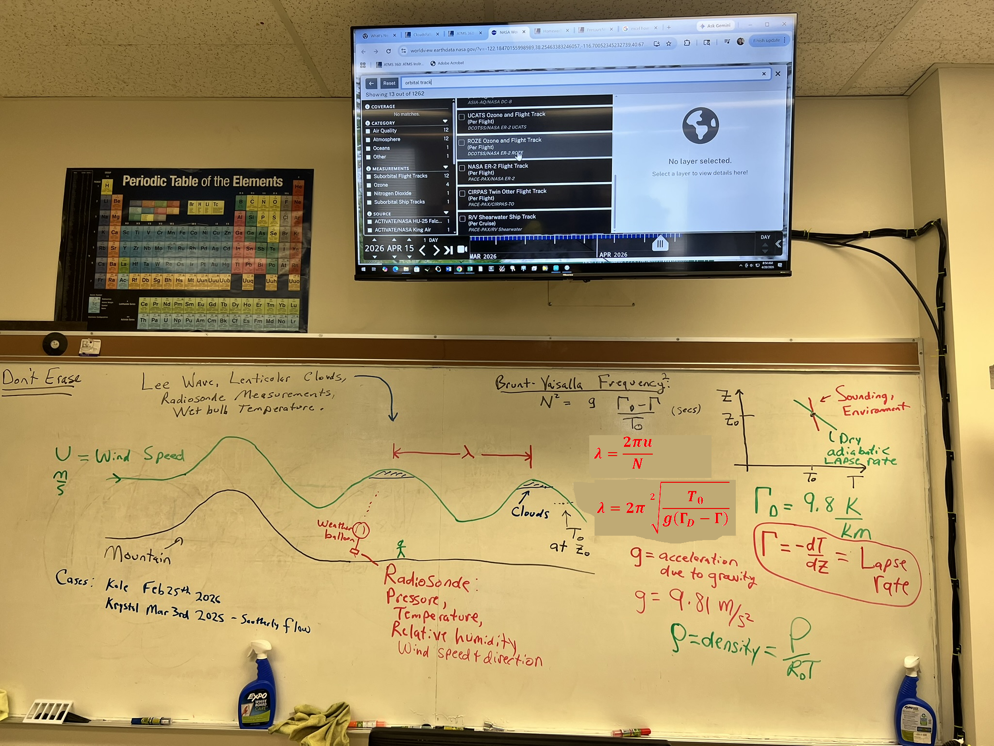
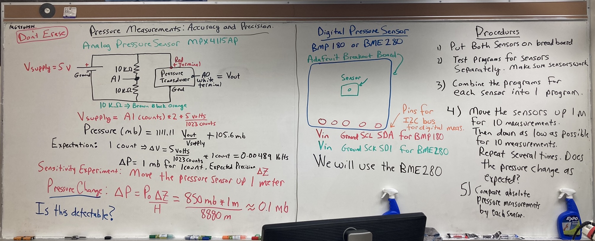
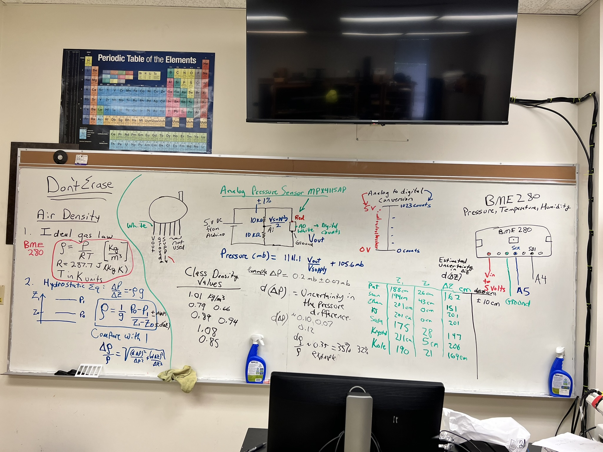
Whiteboard notes of lee wave study.
This meteorological model output may help understand the weather conditions for the day and time leading up to the wave cloud you're working with. Choose the time and date of your sounding and view the various pressure levels of the atmosphere and the various meteorological fields like relative humidity.
Balloon-based sounding presentation.
Waves in the atmosphere presentation. See especially slides 6-28.
Slide Mountain weather station data relevant to observing the atmopsheric pressure near the crest of the Sierra Nevada Mountains nearby Reno.
Slide mountain weather station observed on Google Earth Online.
Radiosonde discussion.
See https://www.weather.gov/upperair/Study2 for radiosonde errors discussion.
See
https://en.wikipedia.org/wiki/Lee_wave for lee wave discussion.
Chase gravity waves to improve weather and climate models.
Observed and Modeled Mountain Waves from the Surface to the Mesosphere near
the Drake Passage
Assignment 9 Analog and Digital Pressure Sensors
Pressure measurements are very important in Atmospheric Science.
Preparation: Make an account with Tinker Cad. We will use this to learn how to work with microcontrollers, sensors, and electronics.
Procedure for pressure sensor measurements.
Use CoolTerm to save data for the following measurements in parts A-D.
Note with Cool term you can start capture to text file before connecting to the Arduino, so you can capture the data information.
|
Evaluate sensor stability by doing measurements over several days.
A. We're ready to test the sensors for use in a weather station.
Set up the computer so it doesn't go to sleep.
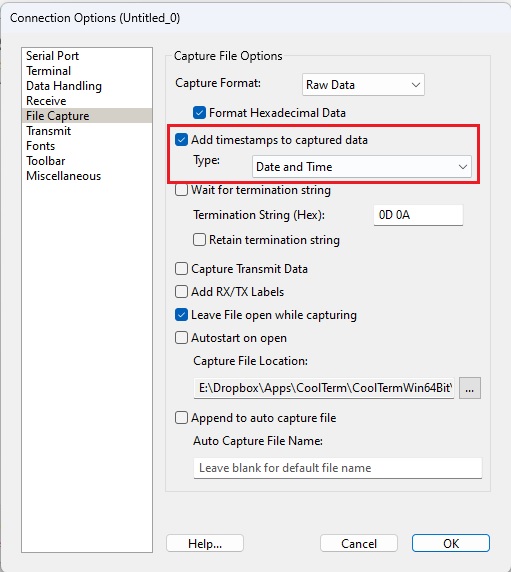
Write the time and date to the file with CoolTerm also for measurements over several days (here's how).
Set CoolTerm to start recording data to a text file.
Connect CoolTerm to the Arduino so that it will stream measurements to the computer until recording data to text file is ended.
Calculate pressure averages in Excel for both the BME280 and the analog pressure sensors. Get a calibration factor for the analog pressure sensor=(Average BME280 Value)/(Average Analog Sensor Value).
Change the pressure calibration factor variable, in the sketch near the top, from 1.0 to the value you obtained.
Upload your program to the Arduino.
Both pressure sensors should measure close to the same value after this.
Make a new column for calibrated ambient pressure. Apply the calibration factor to it.
Calibrated Analog Pressure = Measure Analog Pressure
* (Average BME280 Value)/(Average Analog Sensor Value).
The Calibrated Analog Pressure will be used in all of the graphs.
Make a time series graph with time in minutes on the x axis, with pressure from both sensors on the first y axis, and temperature on the 2nd y axis.
Observe anything of interest, especially if temperature changes correlate with pressure changes. (1st graph).
HINTS ON GETTING DATA INTO EXCEL AND REMOVING BLANK ROWS:
1. Importing into Excel: Read in delimited text: Include delimiters "space" "Tab" and "Comma".
2. Get rid of the empty rows:
a) Click on the first column to select the entire column (click on the A. The whole column should be highlighted)
b) Home:Find & Select (it's on the far right):Go to special:Blanks:OK (This should select only the rows with nothing in them)
c) Home:Delete:Delete sheet rows (This should delete only the rows that had nothing in them)1. Importing into Excel: Read in delimited text: Include delimiters "space" "Tab" and "Comma". |
| |
Evaluate the precision and accuracy of the pressure sensors by their ability to measure small pressure changes.
Use CoolTerm to save data to a file for graphing with Excel.
B . Do measurements with 1 second time average, holding
the sensor 1 meter below the table top for 10 seconds, then up 1 meter above the table top for 10 seconds. Repeat this cycle at least 4 times, with a single data file (each cycle does not need its own data file). Meter sticks are available. If you can't lift move it a full meter up or below the table, record approximately how high or low it can be moved. (2nd graph).
Time in miliseconds is x axis, y axis is pressure for both sensors.
|
| |
Investigate the effect of averaging time on accuracy and precision.
Use CoolTerm to save data to a file for graphing with Excel.
C. Then modify the code to obtain 10 second time averages. Test by holding the sensor low for 100 seconds, and high for 100 seconds.
Repeat this cycle at least twice. (3rd graph).
Time in miliseconds is the x axis, y axis is pressure.
|
Topics to include in your report
Introduction:
Part of this lab is to compare pressure measurements from two sensors.
Briefly discuss what is meant by 'accuracy' and 'precision' in respect to measurements to start the conversation about sensor measurement comparisons. Helpful presentation for this discussion.
Methods:
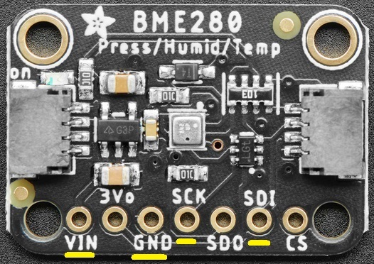
How do these pressure sensors work? It is a good starting point to look at the data sheets for the analog sensor and for the digital sensor and other information on the pressure page. The Freescale MPX4115AP and BME280 use a piezoresistive strain gauge for sensing pressure. Freescale is an analog sensor so the Arduino is doing the analog to digital conversion, requiring a number of hookup wires and components on the breadboard and to Arduino. The BME280 is a digital sensor, so the analog to digital conversion is accomplished within the component itself. Arduino just asks the BME280 for measurement values, and I2C communcations is used for the communication between them. The BME280 also reports temperature and relative humidity and a calculated pressure altitude (altitude determined from a pressure measurement.)
Results:
Use the figures created from measurements described in the Procedure below to answer the following questions.
Looking at the data from Part A, what is an estimated uncertainty in the measurements with each sensor? Do the two pressure sensors measure the same pressure value within the specifications given in their data sheets?
Are the pressure sensors precise enough to show the pressure difference between when the sensors are held high and held low (about a 2 meter difference in height? Are the pressure differences accurate, that is, close to the estimated value of about 0.10 mb/meter?
Compare the fluctuations of the pressure data measured at 1 second intervals versus 10 second intervals. How does averaging time affect the sensor's uncertainty?
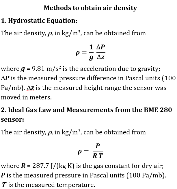
Use your data to calculate the air density from the two methods given here, as an image and as a document. Compare.
|
Note on the analog sensor: It seems the 10 bit analog to digital (a/d) converter of the Arduino would not be able to resolve a pressure difference of about 0.1 mb associated with 1 meter height difference. 1 bit change in the a/d counts corresponds to a voltage change of about 0.005 volts, and a pressure change of and about 1 mb pressure.
Dither helps: the voltage source for the Arduino is noisy enough to cause around 50 mv or so of noise so that the a/d counts fluctuate to a useful average.
The example sketch for pressure averages the measurements of the pressure sensor voltage and the voltage divider voltage about 1800 times for each measurement.
Use of the voltage divider for the power supply voltage measurement is necessary since the a/d range is 5 volts, and direct measurement might be at or over the measurement range.
-->
Assignment 8: Radar Meteorology Application
The goal is to develop skill in working with meteorological radar data.
This assignment works with precipitation and Doppler data from NEXRAD radar.
Practice giving presentations of meteorological data.
Become familiar with commonly used meteorological data.
This is a two part assignment that will be placed in a single powerpoint presentation:
Part 1: An in depth view of a radar, its location, and recent data from it.
Part 2: A case study demonstrating acquistion and interpretation of archived radar data for the same or another radar location.
Deliverables:
A. Presentation turned in through webCampus as a Powerpoint document. (50 points possible)
B. Deliver your presentation to the class. (50 points possible)
A note about time conversion. This site describes how to convert time in UTC to local time (scroll down to get specific instructions). For example, Reno is in the Pacific Standard Time (PST) Zone so that a local storm happening at 10:00 am PST corresponds to time UTC=PST+8 hours=18:00z. The 'z' is added to the time to indicate UTC.
Part 1: Introduction
Choose a radar. Here's where to choose the radar.
It's best to find a radar site that has active precipitation going on so that you can see data from it.
Find the coordinates of your radar for locations in the continental US (for Alaska, Hawaii, etc you'll need to estimate the coordinates).
Presentation Contents Part 1:
1. Put your radar coordinates into Google Earth and make an image of the location of the radar.
Using Google Earth, place circles centered on your image having a radius of 50 and 100 nautical miles, to represent the range of the radar and help interpret the images in parts 2 and 3.
2. Get a GIF movie of 24 images of base reflectivity data from your radar a day when precipitation is present.
Use the Save Data tab to make and save the GIF movie.
3. Get a base velocity 24 image GIF movie of base velocity for the same time.
Use the Save Data tab to make and save the GIF movie.
4. Get a correlation coefficient 24 image GIF movie of the base correlation coefficient for the same time.
Use the Save Data tab to make and save the GIF movie.
Discuss the location of your radar, in particular, any challenges that come about due to location.
Discuss the dbZ level of your base reflectivity GIF movie. Is it large or small, associated with rain and/or snow?
Discuss your base velocity GIF movie, interpreting wind direction and speed.
Discuss your correlation coefficient GIF movie, interpreting the values.
Part 2: Application
Find the time and location of a notorious weather event from anywhere in the continental US at a time when radar data is available. Be sure to note the local time and the 'Coordinated Universal Time' (UTC) time. Possibilities include tornados, hurricanes, derechos, severe thunderstorms, outflow boundary from convective storms, pyrocumulus clouds and/or fire tornados during wildland fires.
Email me the date, time, and location of the event you want to use.
I'll let you know right away if it is suitable and to make sure no one else is doing the same case study.
First, using the date and time in UTC for your event, go to the archived radar data page to be sure your location and time actually has an active storm. This is to make sure that you have the right day, time and location for your weather event, though including this this data in your presentation is optional.
Second, use the NOAA Weather and Climate Toolkit to get the data from the radar closest to your event; obtain animations over the event for reflectivity, radial velocity, and correlation coefficient.
Step by step instructions are given below under Resources for the NOAA Weather and Climate ToolKit (WCT) NEXRAD radar data and animation.
Presentation Contents Part 2:
5. Describe your notorious event.
6. Describe the radar location for your event as in Part 1.
7. Show the radar reflectivity movie for your notorious event and interpret it. Discuss any observational challenges that could have affected radar data, such as beam blocking, etc.
8. Show the radar Doppler velocity movie for your notorious event and interpret it.
9. Show the radar
correlation coefficient movie for your notorious event and interpret it.
10.Show and discuss the HYSPLIT model 2-day-back-trajectory for air arriving at 100 meters above the Earth's surface (AGL) at the tornado, etc location. (Time zone discussion).
Discuss your notorious event and the data from it.
Resources for Software Tools
Install Google Earth, or use it with a browser.
Install Powerpoint or use it from a browser, or use Google Docs, or Pages on the Mac. Students can download Microsoft Office for free through Office 365.
It may be useful to also explore the National Weather Service radar site.
NOAA Weather and Climate Toolkit to obtain past data.
Resources for Radar Understanding:
Great discussion of radar and its applications. (local backup)
Radar discussion.
Interpretation of the radar correlation coefficient. (local backup).
National Weather Service discussion of radar, and another more in-depth discussion.
High windspeed problems with the nexrad radar due to aliasing. Equations and text backup.
Range folding in radar echos.
Resources for Notorious Weather Events:
Case study of a severe storm analyzed by radar.
Tornado discussion.
Tornados in the US since 1950, also given by year when you scroll down and click on a year link.
Strong hurricanes that have hit the US.
Detailed Resources for the NOAA Weather and Climate ToolKit (WCT) NEXRAD radar data and animation:
1. After downloading WCT, find the folder it's in and click on the file wct.ext.The first time it runs there will be a caution about the file. Go to 'more information' and allow it to be run.
2. Click on the "NOAA Open Data"
tab.
3.
Select NEXRAD Level-II.
4.
Choose your radar using the pulldown under the Amazon pulldown.
5. Enter the day of your data, keeping in mind that time is in UTC rather than local time. See the note about time above.
6.
Click on "List Files" to list the data for that day.
7. Scroll down the file list to find the time at the start of the event you're working on and click on it. If all day, just click on the first file.
8. Click on the "Load" button near the bottom of the window. This will bring up the first image. Click on the magnifier icon under "File" menu to center the image.
9. That should bring up another small window called "Radial Properties". This is where you choose 'Moment:' which is measurement type, and radar 'Elevation' angle.
10."Radial Properties:Moment" should say "Reflectivity".
11. Go back to the "Data Selector" window and make sure the filename at the start of your event is highlighted. Scroll down to the time when your event ends. Hold down the shift key and click on the file at the time when your event ends. This should highlight all of the relevant files for your case study.
12. Click on the "Animate" button. This will open an anmiation window. Click on the green "Play" button and confirm that you have storm related radar data and not just ground clutter. The dBZ values should be in the green or higher color bars (> 20 dBZ).
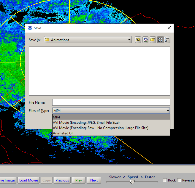
13. While the animation is still running, click on the "Export Movie" button. That will bring up a "Save" window that has pulldowns like this.
14. First try to use the file type "mp4" for export. It is a compressed file type that works well with powerpoint, but WCT has problems with it sometime. If you get an error like this, then follow step 14.a. If not follow step 15. (See step 18 if your animation does not need to be stopped and you want to use "Animated GIF".)
14a. If you get the mp4 error, then choose either the file type "AVI Movie (Encoding:JPEG, Small File Size)" if your movie will be for more than a data extending over 2 hours, or choose "AVI Movie (Encoding Raw - No Compression, Large File Size)" for data extending over less than 2 hours. These AVI files may not be viewable by windows media player, but can be read into powerpoint using this tab and sequence "Insert:VideoThis Device ..", and powerpoint will probably need to format the video. Alternatively, you could use a AVI-mp4 converter like this to get an mp4 video format movie that should be readable by powerpoint.
15. Skip this step if you needed to do step 14a. Otherwise, read your mp4 video into powerpoint using the sequence "Insert:VideoThis Device .." .
16. Click on the video in powerpoint. You can make it start automatically when the slide is presented by using the menu item "Playback:Start:Automatically" and "Loop until Stopped" clicked to show the check mark.
17. Repeat steps 10-16 for "Radial Properties:Moment" =
"RadialVelocity" and then for "Radial Properties:Moment" =
"CorrelationCoefficient" to get their animations into powerpoint.
18. Note:
It is also acceptable to use "Animated GIF" as an animation of your data in step 14 instead of "mp4", especially if your animation does not need to be stopped in to point out specific features.
-->
Assignment 7: Radar Meteorology
The goal of this quick-study active-note-taking discussion is to become familiar with meteorological radar used to detect precipitation and severe weather.
Examples are on this page for composite reflectivity and for the Reno NWS dual polarization radar measurements.
Example of Doppler image for Des Moines Iowa.
Submission is through webcampus. Copy these questions to MS word and work on them.
Be sure to give your sources for answers.
Basics:
1. What is the diameter range for raindrops?
2. What is the diameter range for drizzle drops?
3. What is the diameter range for cloud droplets?
4. What is the shape of raindrops?
5. Why don't raindrops get arbitrarily large?
Local Rain Measurements:
6. What is the rainfall rate equation?
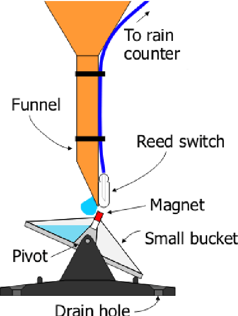
7. How does a simple rain gauge work?
8. How does a tipping bucket rain gauge measure rain? (picture from here).
9. How does a disdrometer work?
National Weather Service Radar.
Weather radar presentation as powerpoint and as a pdf document for understanding radar and dbZ.
10. What is the name of weather radars used by the National Weather Service?
11. What is the wavelength range used by
this radar?
12. Briefly, how does radar work to measure rain?
13. Calculate the size parameter x=2 pi * Raindrop Radius / radar wavelength.
14.
What 'radiation regime' is the size parameter of question 13? Note that it is the same radiation regime that gives rise to the blue sky on a clear day. Note.
15.
What is the basic relationship for radar backscattering in terms of number of raindrops per volume, back scattering strength, droplet diameter D, and radar wavelength lambda? Note.
16.
Why must the radar be empirically calibrated for rainfall rate given question 15, and question 6?
17.
How does Doppler radar work? What can be detected with it?
18. How does dual polarization radar work, and what can be detected with it?
19. What is the correlation coefficient as used in meteorological radar?
20. What does this correlation coefficient indicate?
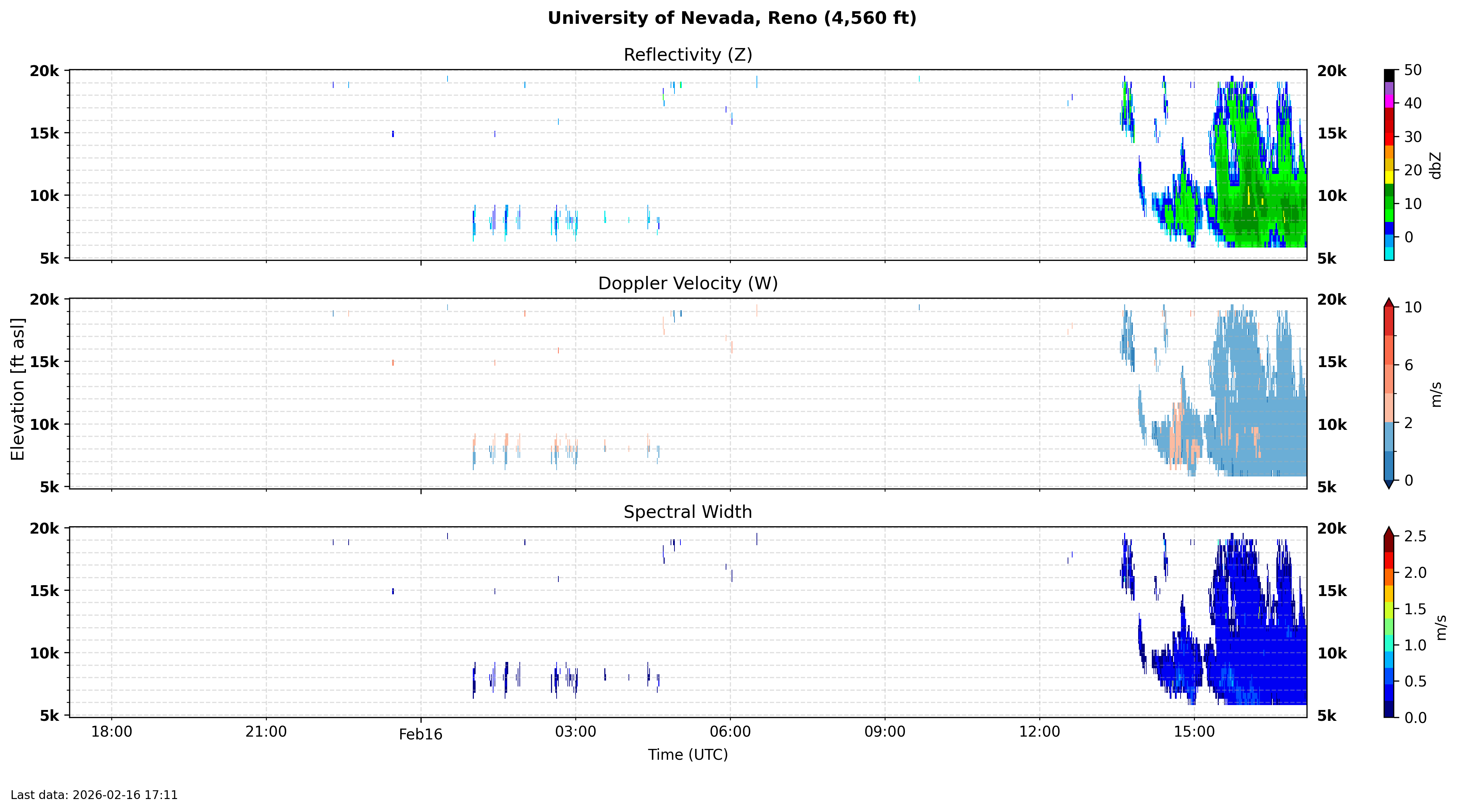
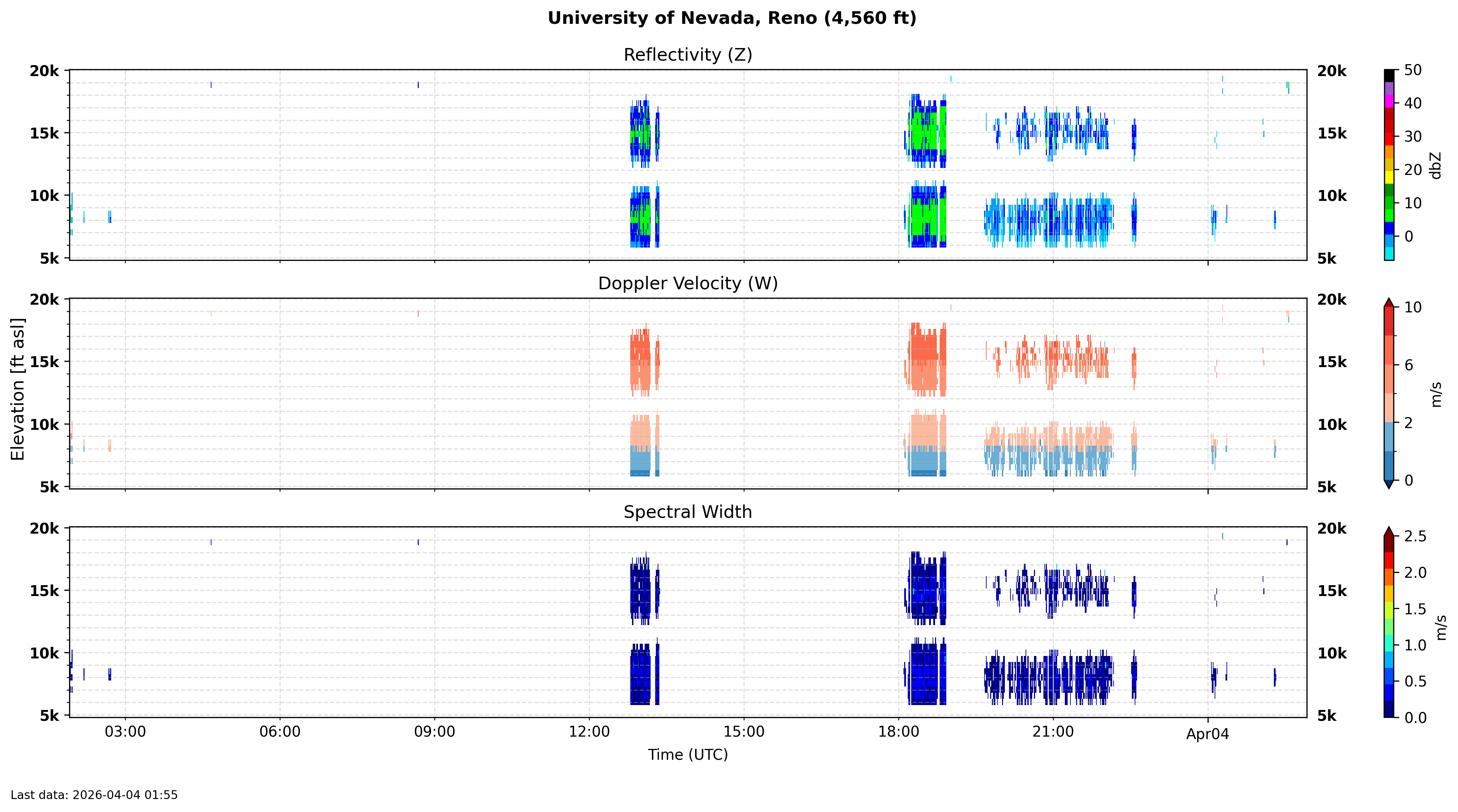
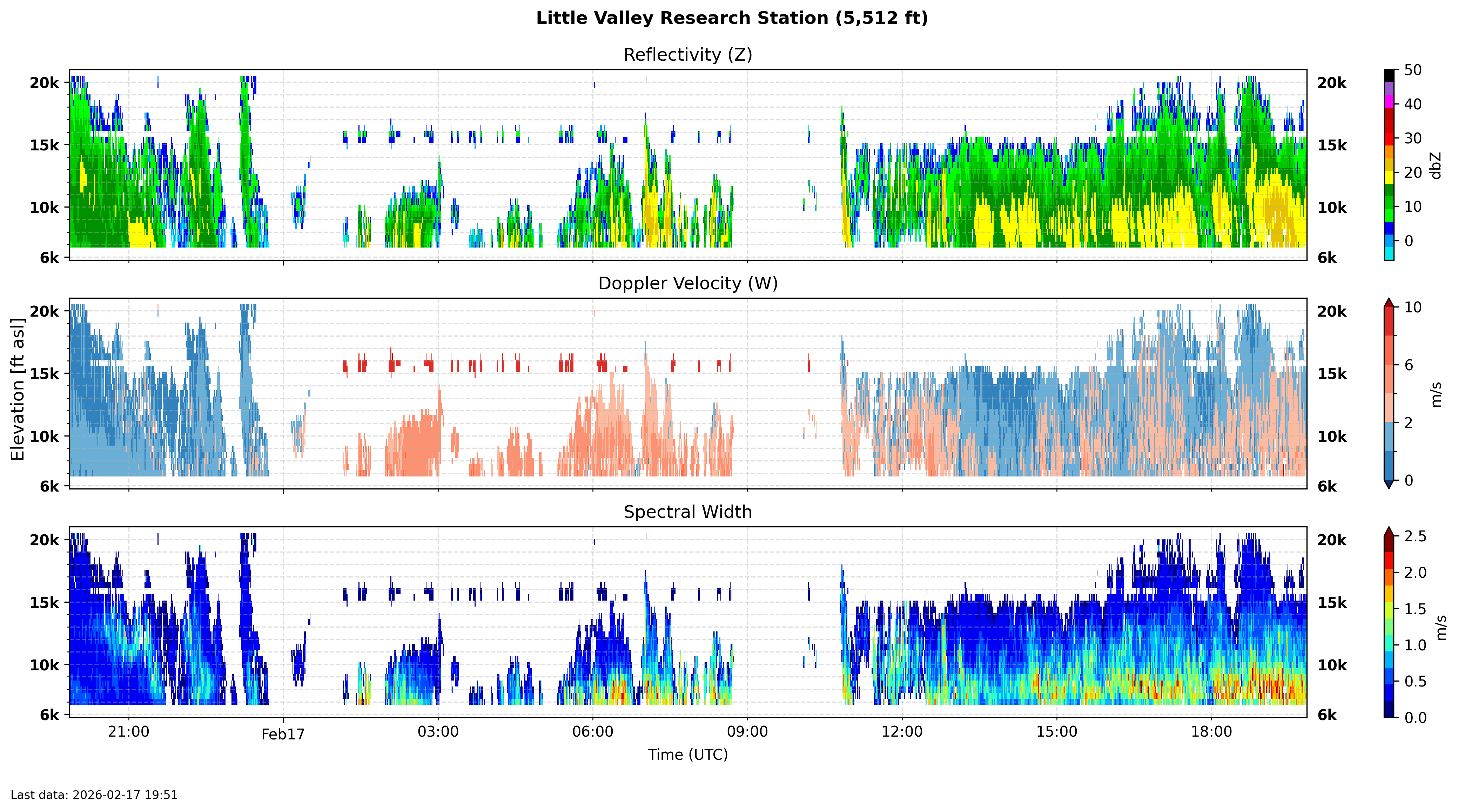
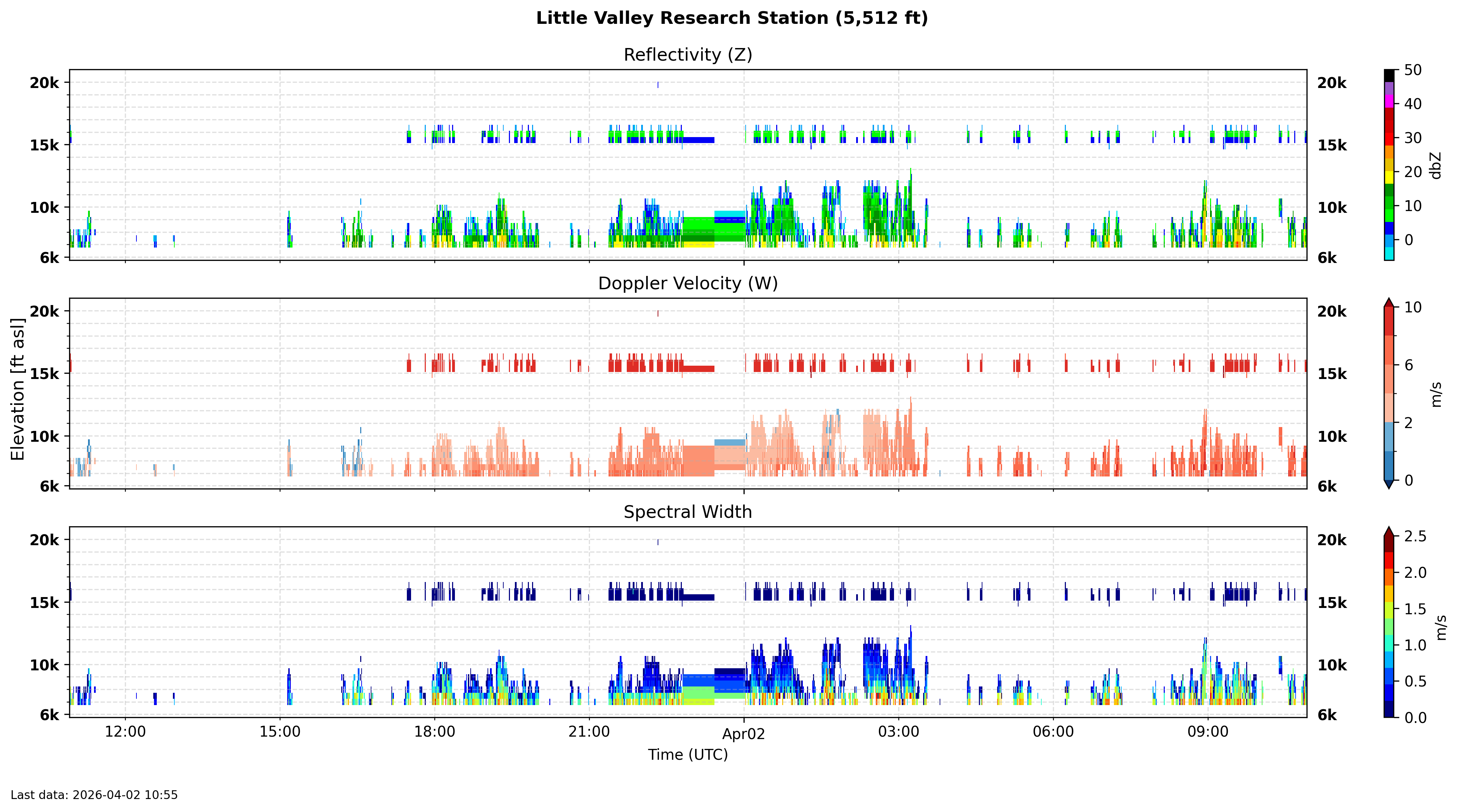
UNR Micro Rain Radar (data example) (Real-time data) LITTLE VALLEY UNR RESEARCH STATION (data example) (Real-time data)
21. What are the wavelength and frequency of MRR-2?
22. Describe the reflectivity, mean Doppler velocity, and spectral width?
23. What is the radar bright band and how can it be determined by the radar?
24. Discuss the reflectivity,Doppler velocity, Spectral Width, and bright band for the Little Valley Research Station data.
Resources:
- Demonstrations and calculations:
a. Fill the aquarium with enough water to use the ultrasonic cloud generator.
b. Make 'raindrops' and have them fall into the aquarium. Note sound made and potential for bubble formation to make more sound.
c. Show the piezo electric sound sensor method of measuring sound droplets. Make a data acquisition system to observe traces created by raindrops hitting the sensor.
d. Calculate how many cloud droplets (diameter d) it would take to make a single raindrop (diameter D). Talk about the lack of ability for radar to 'see' the cloud droplets.
UNR Micro Rain Radar (MRR) current measurements. Little Valley current measurements.
Great discussion of radar and its applications. (local backup).
What's under the dome? Discusses also the rotation of the radar.
Notes on differential polarization and the correlation coefficient associated with it.
National Weather Service discussion of weather radar.
Understanding radar discussion from the weather underground.
-->
Assignment 6: Near-surface weather stations
Purpose:
- Become familiar with near-surface weather stations:
- UNR weather station on Valley Road
- Changes of the surroundings affect the wind measurements?
- Moderately expensive solar-powered weather station with 2D sonic anemometer for wind measurement
(Ambient WS-5000)
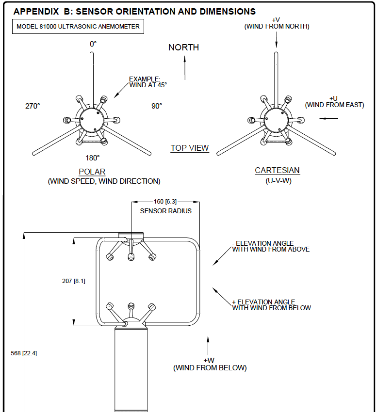
- RM Young 3D sonic anemometer for fast measurements of horizontal wind, pressure, and temperature
- Turbulent kinetic energy and heat flux in addition to 3D wind components.
Lab Report with the Following Contents:
- Part 1:
- UNR weather station on Valley Road
- Use Google Earth (View: Historical) and get images of the UNR weather station for recent and past times. Explain how the area has changed and how that may impact wind measurements.
- Obtain and interpret UNR weather station data for the last 7 days.
- Part 2: (read about measurements of temperature, pressure, and wind)
- Moderately expensive solar-powered weather station with 2D sonic anemometer for wind measurement
(Ambient WS-5000).
- RM Young 3D sonic anemometer for fast measurements of horizontal wind, pressure, and temperature.
- Part 3: Questions for discussion and exploration in your lab report
(read further about lab reports for Atmospheric Sciences)
- What are some of the factors affecting near surface meteorology measurements over many years?
- Asses the WS-5000 weather station measurement accuracy assuming the RM Young 3D sonic anemometer is a measurement standard.
Additional Resources For This Assignment:
1. Style guide for lab reports.
2. UNR and DRI atmospheric instruments and measurement sites.
3. Journal article describing a measurement campaign similar to ours.
4. Atmospheric Instruments Textbook: See Appendix A on lab reports
Free through UNR Library: Online textbook for atmospheric instrumentation.
5. Relationships for wind speed and direction calculations.
6. RM Young sonic anemometer wind direction for U, V, and W winds (horizontal and vertical components).
Related Resources:
7. Wind roses to show wind direction and speed in single graph. (Python script and example data for it from the UNR weather station.)
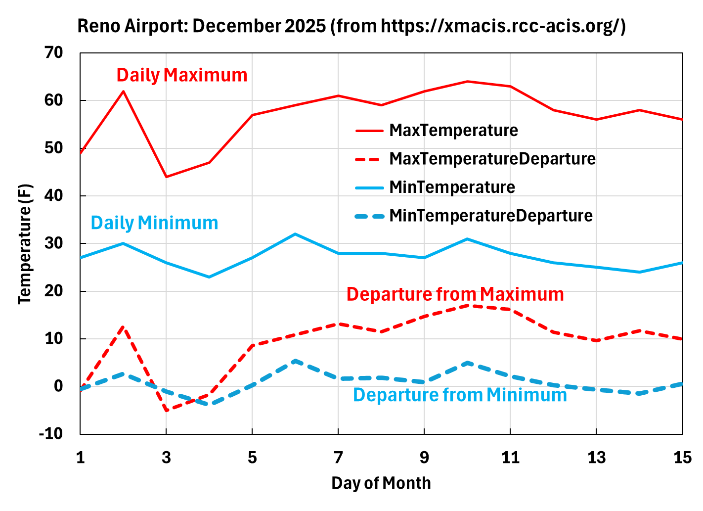
8. Acquire and plot surface weather measurements as a function of time and location. Example of December 2025 minimum and maximum temperatures.
9. Note that tipping bucket precipitation measurements can distort the timing of snow in winter months (snow melts and is measured during day light hours).
Assignments 1 - 5 Online (see webCampus)
Assignment 5 Online (see webCampus) precipitation estimates.
Purpose: Become familiar with precipitation estimate measurements.
Assignment 4 Online (see webCampus) atmospheric radar measurements.
Purpose: Introduction to radar use in meteorology.
Assignment 3 Online (see webCampus) measurement of wind.
Purpose: Become familiar with atmospheric wind measurements.
Assignment 2 Online (see webCampus) measurement of atmospheric temperature.
Purpose: Become familiar with atmospheric temperature measurements.
Assignment 1 Online (see webCampus) Overview of Atmospheric Instrumentation.
Purpose: Broad overview of atmospheric instrumentation measurements.
This is an online homework assignment and is described on webCampus.
(Top of page) .