Week 16: 9 December 2019
Final Project Presentations Finish up.
Class evaluation is open, please do so before December 11th.
The in-class final exam is on Thursday December 12th from 9:50 am to 11:50 am.
You can bring an equation sheet, 8.5" x 11" with notes on front and back.
Bring your calculator. 80% of final.
The in-class portion covers atmospheric thermodynamics and radiation, chapters 1, 3, and 4.
The take home portion will be assigned that day too, see webcampus on December 10th for the problems. 20%
The take home portion covers cloud physics, chapters 5 and 6, and will be due at the latest December 17th at the end of the day.
Plan for this week:
Continue Aerosol and Cloud Microphysics:
This article is a current update on cloud and aerosol related microphysics and is easy to read. Read it first.
Then read chapter 6 on cloud microphysics from Wallace and Hobbs. We will discuss parts of chapter 5 to help with chapter 6.
Cloud and aerosol physics presentation.
Final Exam Notes:
Final Exam Practice Problems. Note that some of the cloud physics problems are relevant to the take home rather than in class portion of the final.
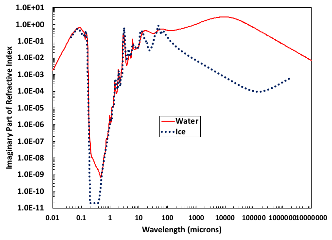
Radiation transfer topics include those in chapter 4, and those from homework and lecture; how to use the size parameter to identify the relevant scattering regime and how to calculate scattering cross sections in these limits; direct and diffuse radiation in the atmosphere; real and imaginary parts of the refractive index; electromagnetic penetration depth and volume versus surface absorbers.
Skew T practice: Problems 3.37, 3.45, 3.47, 3.48, 3.53, Solutions to check your work are here. The skew T as a gif file is here.
More practice problems with solutions are here. Skew T tutorial is here.
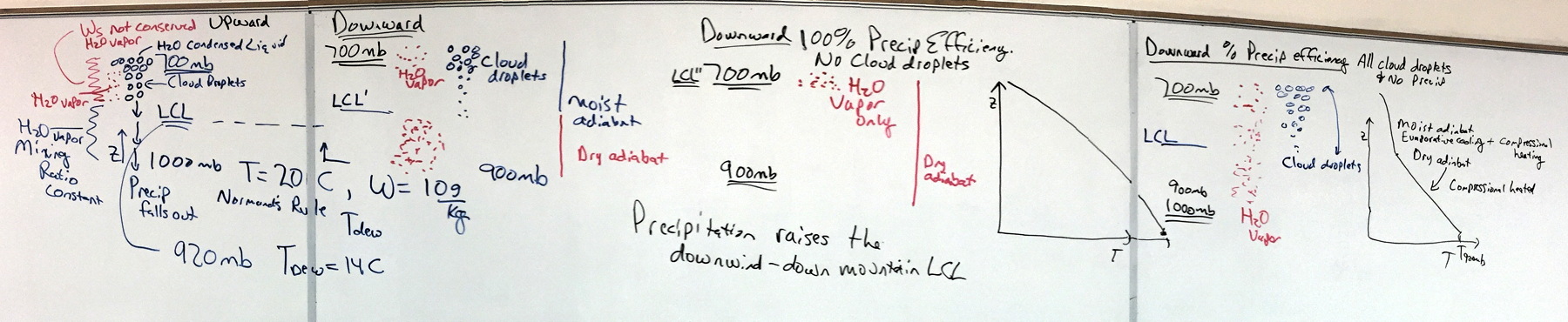
Problem 3.48 Air going over a mountain range and temperature effects due to precipitation: Chinook winds. (review, good for adiabatic liquid water content too).
Previous Midterm Exams for practice, that were posted earlier in the semester:
Here are two previous exams to use for style and study. Exam 1. Exam 2.
Week 15: 2 December 2019
DECEMBER 4th Final Project Presentations Start:
Reread the final project assignment; you can work on it all semester. The end of the semester approaches.
Presentations begin on December 4th for projects.
The in-class final exam is on Thursday December 12th from 9:50 am to 11:50 am.
You can bring an equation sheet, 8.5" x 11" with notes on front and back.
Bring your calculator. 80% of final.
The in-class portion covers atmospheric thermodynamics and radiation, chapters 1, 3, and 4.
The take home portion will be assigned that day too, see webcampus on December 10th for the problems. 20%
The take home portion covers cloud physics,
chapters 5 and 6, and will be due at the latest December 17th at the end of the day.
Plan for this week:
Start Aerosol and Cloud Microphysics:
This article is a current update on cloud and aerosol related microphysics and is easy to read. Read it first.
Then read chapter 6 on cloud microphysics from Wallace and Hobbs. We will discuss parts of chapter 5 to help with chapter 6.
Cloud and aerosol physics presentation.
 |
 |
 |
Related Information
NASA undergraduate scholarship program
SUMMER INTERNSHIP OPPORTUNITY IN PARALLEL COMPUTING IN ATMOSPHERIC SCIENCE
Snow flake from Sunday morning.
Winter microphysics processes.
Magono Lee ice crystal classification system.
Ice crystal habit and super saturation.
Week 14: 25 November 2019
Reread the final project assignment; you can work on it all semester. The end of the semester approaches.
Plan for this week:
Continue with chapter 4.
Bring questions on Homework 8 to class on Monday.
Single and multiple scattering, and transmission and reflection of solar radiation by clouds above a reflecting ground.
Transmission and reflection by clouds, and clouds above the ground.
Model for maximum diffuse radiation as a function of optical depth.
Reference reading material from here for the multiple scattering model used for cloud transmission.
Slide 52: Radar backscatter efficiency for ice and water spheres are 10.7 cm radar wavelength, radar remote sensing of precipitation.
Slides 26-33: Solar radiation at the top of the atmosphere and at the surface: Aerosol and gaseous absorption and scattering impacts.
Slides 34-35: Line broadening.
Slides 36-49, radiative heating rate of the atmosphere, low and high cloud radiative forcing, and spectral upwelling and downwelling longwave radiation.
Start Cloud Microphysics:
This article is a current update on cloud and aerosol related microphysics and is easy to read. Read it first.
Then read chapter 6 on cloud microphysics from Wallace and Hobbs. We will discuss parts of chapter 5 to help with chapter 6.
Cloud and aerosol physics presentation.
 |
 |
 |
 |
 |
 |
 |
 |
|
 |
 |
Related Information
SUMMER INTERNSHIP OPPORTUNITY IN PARALLEL COMPUTING IN ATMOSPHERIC SCIENCE
Mie Theory Calculator for electromagnetic scattering by spherical particles.
Graupel particle from Monday morning.
Ice nuclei discussion.
Lab experiment demonstrating ice crystal multiplication, and related paper discussing atmospheric applications.
Smoke interacting with clouds.
Ship tracks.
Week 13: 18 November 2019
Reread the final project assignment; you can work on it all semester. The end of the semester approaches.
Plan for this week:
Continue with chapter 4.
Review scattering and absorption regimes for particles using the size parameter and penetration depth.
Discuss application to scattering of electrons off of atomic nuclei, protons, and quarks (deBroglie wavelength of electrons).
Single and multiple scattering, and transmission and reflection of solar radiation by clouds above a reflecting ground.
Transmission and reflection by clouds, and clouds above the ground.
Model for maximum diffuse radiation as a function of optical depth.
Reference reading material from here for the model we'll be using.
Homework assignment 8.
Slides
54-66, single and multiple scattering ideas, leading up to transmission through clouds.
Slides 74-86, Rayleigh scattering, Mie (resonance) and geometrical optics scattering regimes.
Slides 36-49, radiative heating rate of the atmosphere, low and high cloud radiative forcing, and spectral upwelling and downwelling longwave radiation.
Slide 50, demonstration of light transmission using a dilute solution of milk in water.
Plan for next week after Homework 8:
Start cloud microphysics.
This article is a current update on cloud and aerosol related microphysics and is easy to read. Read it first.
Then read chapter 6 on cloud microphysics from Wallace and Hobbs. We will discuss parts of chapter 5 to help with chapter 6.
 |
 |
 |
 |
 |
 |
 |
 |
 |
 |
 |
 |
 |
Related Information
SUMMER INTERNSHIP OPPORTUNITY IN PARALLEL COMPUTING IN ATMOSPHERIC SCIENCE
Mie Theory Calculator for electromagnetic scattering by spherical particles.
Diffraction in the atmosphere.
When will it snow? Mackay miner.
Rainfall measurement by radar and attenuation.
Rainfall rate measurement by attenuation of microwave sources.
Derivation of the 2 stream model for radiation transfer.
Ice cloud microphysics: Ice multiplication mechanism (Hallett Mossop process) and review.
Week 12: 12 November 2019
Reread the final project assignment; you can work on it all semester.
NASA Worldview
Mie Theory Calculator for electromagnetic scattering by spherical particles.
Diffraction in the atmosphere.
When will it snow? Mackay miner.
Plan:
Continue with chapter 4.
1 layer model for atmospheric transmission including solar absorption and infrared absorption and emission.
Cross sections for absorption, scattering, and extinction.
Absorption, scattering, and extinction coefficients and optical depths and relation to atmospheric transmission.
Electromagnetic penetration depth and attenuation of wireless signals by rain and snow (see below too).
Homework assignment 7.
Transmission and reflection by clouds, and clouds above the ground.
Model for maximum diffuse radiation as a function of optical depth.
Reference reading material from here for the model we'll be using.
Homework assignment 8.
Slides 14-16, 1 layer model of the atmosphere with solar absorption and longwave absorption and emission.
Slides
54-66, single and multiple scattering ideas, leading up to transmission through clouds.
Slides 74-85, Rayleigh scattering, Mie (resonance) and geometrical optics scattering regimes.
Slides 36-49, radiative heating rate of the atmosphere, low and high cloud radiative forcing, and spectral upwelling and downwelling longwave radiation.
Slide 50, demonstration of light transmission using a dilute solution of milk in water.
 |
 |
 |
 |
 |
 |
 |
 |
 |
 |
 |
 |
 |
Related Information
Radar chaff fall speed and radar return, for understanding false radar echos.
More on radar sensing of precipitation.
Terminal velocity of falling objects.
SUMMER INTERNSHIP OPPORTUNITY IN PARALLEL COMPUTING IN ATMOSPHERIC SCIENCE
Persistent drizzle (liquid water precipitation) at -25 C in Antarctica.
Week 11: 4 November 2019
Reread the final project assignment; you can work on it all semester.
Rayleigh scattering by a sphere of complex refractive index m, wavelength λ, and diameter d,
valid for d<<λ.


Raindrop size distribution discussion (do a radar contribution calculation).
Plan:
Continue with chapter 4.
Review astronomical temperature for the Earth.
Problems 4.21 and 4.29, response of the planet to changes in the solar and infrared radiation.
Homework assignment 6.
1 layer model for atmospheric transmission including solar absorption and infrared absorption and emission.
Cross sections for absorption, scattering, and extinction.
Absorption, scattering, and extinction coefficients and optical depths and relation to atmospheric transmission.
Electromagnetic penetration depth and attenuation of wireless signals by rain and snow (see below too).
Homework assignment 7.
Transmission and reflection by clouds, and clouds above the ground.
Model for maximum diffuse radiation as a function of optical depth.
Reference reading material from here for the model we'll be using.
Homework assignment 8.
Slides
54-66, single and multiple scattering ideas, leading up to transmission through clouds.
Slides 74-85, Rayleigh scattering, Mie (resonance) and geometrical optics scattering regimes.
Slides 36-49, radiative heating rate of the atmosphere, low and high cloud radiative forcing, and spectral upwelling and downwelling longwave radiation.
Slide 50, demonstration of light transmission using a dilute solution of milk in water.
|
 |
 |
 |
 |
 |
 |
 |
 |
 |
 |
 |
Week 10: 28 October 2019
Reread the final project assignment; you can work on it all semester.
Thursday:
Astronomical temperature for the Earth.
1 layer model for atmospheric transmission including solar absorption and atmospheric transmission.
Cross sections for absorption, scattering, and extinction.
Absorption, scattering, and extinction coefficients and optical depths and relation to atmospheric transmission.
 |
 |
 |
Wednesday:
Students present HW5 problems.
Tuesday:
Infrared camera demonstration of optical properties of materials, and heat conduction and convection.
Glasses and glass plate: transparent for visible radiation, strong absorber and emitter of longwave radiation.
Aluminum foil: Strong reflector of longwave radiation, very weak absorber and emitter.
Skin: Strong absorber and emitter of long wave radiation.
Black trash bag: nearly transparent to long wave radiation.
Discussed also the downwelling short and long wave radiation data measured at the UNR weather station this last week.
 |
Monday:
Continue with chapter 4, radiation transfer (presentation).
Bring questions about HW 5 to class for discussion.
Calculator for blackbody radiation.
|
|


Questions for review:
1. Given these two figures, how can we ever get a radiation balance for the Earth? (see the magnitude of the radiation from each source).
2. What are wavelengths for the peaks on each?
3. The two graphs below are the downwelling solar and infrared radiation for the last 7 days from the UNR weather station.
Interpret times of clear and cloudy skies, and the atmospheric temperature.
 Downwelling solar radiation for the last 7 days. |
 Downwelling infrared radiation for the last 7 days. |
 Air temperature for the last 7 days. Air temperature for the last 7 days. |
 |
 |
 |
Week 9: 21 October 2019
Monday: Midterm exam.
Tuesday:
Mixing air parcels of different vapor pressure and temperature to get a supersaturation, relevant to condensation nuclei counters as well, slides 91-93.
Look for gravity waves in clouds, Saturday October 19th, 2019, or so should be good.
Formation of gravity waves in the atmosphere and associated clouds (slides 126-147).
Wednesday:
Sound propagation in the atmosphere as affected by the lapse rate, and when thunder no longer can be heard (slides 149-152).
Project ideas and more on waves in the atmosphere.
Use NASA World view to illustrate imagery from the following.
Polar orbiter, NASA AQUA and TERRA satellites, MODIS instrument (705 km orbit diameter) showing gravity waves from 22 Oct 2019.
Geostationary satellite imagery GOES satellite (orbit diameter 35786 km) and example image showing gravity waves from 22 Oct 2019.
View Guadalupe Island using Google Earth online and MODIS imagery from NASA Worldview for cloud examples of Von Kármán vortex street circulation downwind of the island.
 |
 |
Thursday:
We will begin chapter 4, Atmospheric Radiation. Read problem 4.11 (part 1, part 2) now so that you can think about these questions as you read chapter 4.
Homework 5 will be posted.
Online homework will be posted.
 |
Related Information
Undergraduate research internship opportunities in Atmospheric and Space Science through the National Science Foundation.
Atmospheric models (for example Thermodynamics, NAM3k, mlCAPE; vertical cross section of in plane wind).
 |
Week 8: 14 October 2019
Thursday: Review problem 3.48 and variations, slide 60.
Mixing air parcels of different vapor pressure and temperature, slides 91-93.
Look for gravity waves in clouds.
 |
 |
Wednesday: Practice with the skewT. Review dewpoint, wetbulb temperature, and Normand's rule (slides 88-90)
Skew T showing definition of the lines on the chart:
The skew T as a gif file is here (without the definitions).
Tuesday: Homework 4 presentations continue.
Then discussion of water vapor and condensed water.
LFC and LCL (slide 62).
Dewpoint, wetbulb temperatures, saturation vapor pressure difference for ice and water, and mixing dry and moist air parcels to achieve saturation (slides 85-93).
Formation of gravity waves in the atmosphere and associated clouds (slides 126-147)
Sound propagation in the atmosphere as affected by the lapse rate, and when thunder no longer can be heard (slides 149-152).
Homework 4 due on Monday. Finish up chapter 3 and prepare for the midterm exam.
Midterm Exam Prep For Exam on Monday 21 Oct 2019:
Here are two previous exams to use for style and study. Exam 1. Exam 2.
You can use an equation/note sheet, one side, 8 1/2" by 11", for the exam.
More Skew T practice: Problems 3.37, 3.45, 3.47, 3.48, 3.53, Solutions to check your work are here. The skew T as a gif file is here.
More practice problems with solutions are here. Skew T tutorial is here. Problem 3.48 is discussed here.
Procedures for obtaining useful quantities from skewT graphs.
Discussion of the skew T graph and examples.
Monday Class:
Group presentations for Homework 4 start.
Chapter 3 topics
Read chapter 3, Atmospheric Thermodynamics. We will have several homework assignments from this especially important chapter.
Presentation for chapter 3.
The goals (learning and review objectives)
a. Ideal gas equation applied to dry and moist air.
b. Virtual temperature.
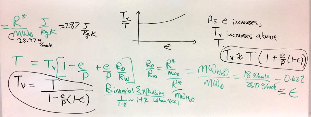
c. Potential temperature.
d. Hydrostatic equation.
e. Increasingly detailed description of the temperature and pressure distribution in the atmosphere.
f. SkewT logP diagrams.
f-g. Relative humidity, absolute humidity.
g. Dew point temperature.
h. Wet bulb temperature.
i. Equivalent potential temperature.
j. Latent heat release and absorption in condensation and evaporation of water.
k. Stability of air parcels.
l. Indices on soundings.
m. Brunt–Väisälä frequency and gravity waves.
o. Sound propagation in the atmosphere.
Related Information:
Undergraduate research internship opportunities in Atmospheric and Space Science through the National Science Foundation.
Atmospheric models (for example Thermodynamics, NAM3k, mlCAPE; vertical cross section of in plane wind).
October 17th 3 to 4 pm. Joe Crowley student union theatre. Information Literacy on Complex or Controversial Topics
Meet Gabriela Gonzalez of the LIGO Scientific Collaboration.
She will describe the history and details of this incredible, Nobel-winning discovery.
She will also discuss other exciting observations (including some very recent ones in 2019), and the gravity-bright future of the field.
More than 100 years after Albert Einstein predicted gravitational waves – ripples in spacetime caused by violent cosmic collisions –
LIGO scientists confirmed their existence using large, extremely precise detectors in Louisiana and Washington. Special Appearance:
Thursday, October 17, 12:15-1:15pm, JCSU 324 (Pizza provided)
The College of Science is also hosting Dr. Gonzalez during lunch so students can have the opportunity to hear her "tell her story" as a Latina research scientist.
Discover Science Lecture Series:
Thursday, October 17, 7pm, DMSC 110

Thursday October 17th talk in the DMS Auditorium.
See also the movie! Look especially at the latter part of the day. And notice the halos present. |
 Image in Google Earth to get wavelength. |
 |
 From here. The original article is here. |

Week 7: 7 October 2019
Thursday Class:
 |
Discuss preparation of soundings for HW4, coloring them for CAPE and CIN, and obtaining 500 mb NCEP reanalysis data for the day and time of your sounding.
Identify your sounding before class, and be ready to use it in class.
Example sounding we can work with. Reno 0Z 22 July 2019. Site for viewing archived radar and other meteorological data.
Wednesday Class:
Be prepared to work with your sounding with CAPE and work with your group towards homework 4.
We will also briefly discuss a correction to problem 3.48, and slides 141 and 142, conditional and convective instabilities,
and the condition for convective instability, dθE/dz < 0.
Also talk about CAPE and precipitable water, slides 74-77.
Monday class:
Discuss and work on HW3. (originally this was going to be a quiz, but changed in webcampus to Homework 3).
Bring questions to class.
Skew T for problem 3.48 example we'll do in class.
Skew T showing definition of the lines on the chart:
Homework 4 has been posted. It is on the topic of soundings related to deep convection.
Read section 8.3.1a, pages 344-347, on deep convection.
This is a group project.
Example sounding.
We will be doing work on this assignment during class this week.
Reread the final project assignment; you can work on it all semester.
Plan:
Continue working on atmospheric thermodynamics, working towards the next homework assignment.
 |
 |
 |
 |
 |
 |
 |
 |
 |
 |
 |
 |
 |
 |
 |
Chapter 3 topics
Read chapter 3, Atmospheric Thermodynamics. We will have several homework assignments from this especially important chapter.
Presentation for chapter 3.
The goals (learning and review objectives)
a. Ideal gas equation applied to dry and moist air.
b. Virtual temperature.
c. Potential temperature.
d. Hydrostatic equation.
e. Increasingly detailed description of the temperature and pressure distribution in the atmosphere.
f. SkewT logP diagrams.
f-g. Relative humidity, absolute humidity.
g. Dew point temperature.
h. Wet bulb temperature.
i. Equivalent potential temperature.
j. Latent heat release and absorption in condensation and evaporation of water.
k. Stability of air parcels.
l. Indices on soundings.
m. Brunt–Väisälä frequency and gravity waves.
o. Sound propagation in the atmosphere.
Related Information:
Atmospheric models (for example Thermodynamics, NAM3k, mlCAPE; vertical cross section of in plane wind).
October 17th 3 to 4 pm. Joe Crowley student union theatre. Information Literacy on Complex or Controversial Topics
Week 6: 30 SeptemberThursday class: Discuss and work on HW3. (originally this was going to be a quiz, but changed in webcampus to Homework 3).
Reread the final project assignment; you can work on it all semester.
Atmospheric models (for example Thermodynamics, NAM3k, mlCAPE; vertical cross section of in plane wind).
Plan:
Continue working on atmospheric thermodynamics, working towards the next homework assignment.
Homework 3 part 1 (analytical questions) are due on the 29th of September.
A new online homework assignment has been posted.Chapter 3 topics
Read chapter 3, Atmospheric Thermodynamics. We will have several homework assignments from this especially important chapter.
Presentation for chapter 3.
The goals (learning and review objectives)
a. Ideal gas equation applied to dry and moist air.
b. Virtual temperature.
c. Potential temperature.
d. Hydrostatic equation.
e. Increasingly detailed description of the temperature and pressure distribution in the atmosphere.
f. SkewT logP diagrams.
f-g. Relative humidity, absolute humidity.
g. Dew point temperature.
h. Wet bulb temperature.
i. Equivalent potential temperature.
j. Latent heat release and absorption in condensation and evaporation of water.
k. Stability of air parcels.
l. Indices on soundings.
m. Brunt–Väisälä frequency and gravity waves.
o. Sound propagation in the atmosphere.
Stability for sounding analysis; review of stability using potential temperature; introduction equivalent potential temperature; isentrope discussion for vertical cross sections.
Wednesday Class: Crucial discussion of the dry adiabtic lapse rate, potential temperture, the vertical distribution of potential temperature, and stability of the atmosphere. Quiz announced (see second image) see webCampus and the homework website. This will actually be HW3 rather than a quiz.
Tuesday Class: Cp and Cv relationship, dry adiabatic lapse rate, and potential temperature.
Monday Class: Thermodynamic processes, first law of thermodynamics, and calculation of the isochoric specific heat at constant volume from the equipartition theorem.
Related Information:
Meteorological analysis using isentropes (constant potential temperature surfaces) and local backup.
The National Weather Center Research Experience for Undergrads program is accepting applications.
Student chapter of the AMS meteorology club meeting Monday at 1 pm in Leifson Physics conference room, RM 208.
Lenticular clouds observed on Friday the 27th. Tis the season.
October 1st Morning looking towards the sun. Pollution buildup due to the morning inversion is evident. Time lapse movie of Saturday Sept 28, 2019, from the Reno National Weather Service Office.
Cold front explanation (from here).
Last 7 days weather at the UNR campus showing the surface pressure, temperature, and wind change with the passage of the cold front on Saturday.
Last 7 days of satellite imagery.
500 mb level on Saturday Sept 28 2019.
Week 5: 23 September
Here's the 500 mb level site we discussed in class on Monday.
The 500 mb level winds are animated here.
Discussion of the 500 mb level.
Additional discussion of the 500 mb level.
Temperature and height of the 500 mb level for Reno Sept 2019. From this spreadsheet.
Observed 500 mb level heights and winds.
Discussion of constant pressure charts.Reread the final project assignment; you can work on it all semester.
Plan:
Bring questions about homework 2 presentations to class on Monday.
Homework 2 analytical problems will be due on 29 September.
Homework presentations on Tuesday. Take good notes for problems discussed by other students.
Chapter 3 topics
Read chapter 3, Atmospheric Thermodynamics. We will have several homework assignments from this especially important chapter.
Presentation for chapter 3.
The goals (learning and review objectives)
a. Ideal gas equation applied to dry and moist air.
b. Virtual temperature.
c. Potential temperature.
d. Hydrostatic equation.
e. Increasingly detailed description of the temperature and pressure distribution in the atmosphere.
f. SkewT logP diagrams.
f-g. Relative humidity, absolute humidity.
g. Dew point temperature.
h. Wet bulb temperature.
i. Equivalent potential temperature.
j. Latent heat release and absorption in condensation and evaporation of water.
k. Stability of air parcels.
l. Indices on soundings.
m. Brunt–Väisälä frequency and gravity waves.
o. Sound propagation in the atmosphere.
Tuesday: Hypsometric equation and a wind speed calculation example at the 500 mb level above Reno.
Monday: Hypsometric Equation and geostrophic wind speed
Week 4: 16 September
Reread the final project assignment; you can work on it all semester.
Plan:
Bring questions about homework 1 to class on Monday. Homework 1 is due at the end of the day.
Continue to work on Homework 1. We had a brief start last Thursday.Where we are headed:
Read chapter 3, Atmospheric Thermodynamics. We will have several homework assignments from this especially important chapter.
Presentation for chapter 3.
The goals (learning and review objectives)
a. Ideal gas equation applied to dry and moist air.
b. Virtual temperature.
c. Potential temperature.
d. Hydrostatic equation.
e. Increasingly detailed description of the temperature and pressure distribution in the atmosphere.
f. SkewT logP diagrams.
f-g. Relative humidity, absolute humidity.
g. Dew point temperature.
h. Wet bulb temperature.
i. Equivalent potential temperature.
j. Latent heat release and absorption in condensation and evaporation of water.
k. Stability of air parcels.
l. Indices on soundings.
m. Brunt–Väisälä frequency and gravity waves.
o. Sound propagation in the atmosphere.
Thursday: Hydrostatic equation and applications: Start layer thickness discussion, hypsometic equation, and pressure levels.
Wednesday: Virtual Temperature. Click image for larger version.
Tuesday: Ideal gas law in its many forms; partial pressure; and the microscopic, kinetic theory of pressure
Model for pressure discussed Monday. Related Information:
McNair Scholars Program at UNR: A program to help you succeed as an undergrad, and in grad school.
AMS scholarships for undergrads and grads, deadlines approaching.
Sudden stratospheric warming in Antarctica, and in general.
Meteor trails and the vertical structure of the atmosphere. (Useful for problem 1.6e).
Week 3: 9 September
Plan:
Continue to work on Homework 1. We had a brief start last Thursday.
Strategy for obtaining the scale height from the sounding data.
Related Information:
AMS scholarships for undergrads and grads, deadlines approaching.
Week 2: 2 September
Plan:
Continue introduction to the skewT diagram and it's uses.
Discuss problem 1.12 on homework 1 to illustrate concepts of chapter 1 through analysis of atmospheric data. Visit Antarctica for example soundings.Skew T showing definition of the lines on the chart: Discuss the trajectory of an air parcel lifted from the surface to the top of the atmosphere.
Clouds and lifting condensation level.
Look at the Reno soundings for 0z and 12z on August 29th as examples of summer time afternoon and morning soundings and interpretation using air density.
8 August 2019 0z sounding and the associated vertical motions as measured by the UNR lidar.
Begin working on problem 3 of the homework.
Water vapor pressure from yesterday and discussion of density for interpretating soundings , and doppler lidar discussion
Wednesday 4 Sept class. Dewpoint temperature and air parcel example from the surface conditions of the Reno morning sounding. Click images for larger version.
Tuesday 3 Sept class. Problem 1.12 discusson and curves on the skew T lnP diagram
Related Information:
Physics seminar on black holes.
Undergraduate Research Scholarship Opportunity: UNR NSF EPSCOR project.
Find a faculty mentor; brainstorm a project; write a proposal; hopefully get funded to carry out the research project, often a good lead in for your senior thesis project.Perlan project in Argentina. Glider out of Minden NV that's going for the world's record altitude in the Andes mtns of Argentina.
Week 1: 26 August
Skew T showing definition of the lines on the chart.
Atmospheric Sounding Data from UWyo.
Thursday 29 August class: Intro to the skewT lnP diagram
Wednesday 28 August class: Density of dry and moist air and variation of temperature with altitude.
Tuesday 27 August class: Pressure and temperature in the atmosphere. Click images for larger version
Monday 26 August class: click image for larger version
First Day Agenda Introductions -- each student introduce themselves and give their major. Syllabus. Homework. Webcampus for online homework assignments/reading.
Required and Optional Course Materials
- Required Textbook: Atmospheric Science: An Introductory Survey by Wallace and Hobbs. Companion site.
- Supplemental Textbook: A First Course in Atmospheric Thermodynamics by Grant W. Petty.
- Article on multiple scattering in the atmosphere.
- Free online Introductory Textbook for Atmospheric Science and local backup
- Skew T presentation for in class discussions and as a gif file to be used with Paint..


Homework 1 is due 10 Sept 2018, to be turned in through web campus as well.
Online Homework 1 is due 1 Sept 2017. See webcampus. This is based on MetEd.
The final project has been posted.
Homework for Monday and Tuesday: Read chapter 1.
This class is:
Related Information:
One part lecture;
One part active class participation/activity involving atmospheric data from around the world;
One part study using online modules for atmospheric science education.
Overview Presentation: Atmospheric Science relies heavily on measurements and models!
Vertical structure of the atmosphere.
Undergraduate Research Scholarship Opportunity: UNR NSF EPSCOR project.
Perlan project in Argentina. Glider out of Minden NV that's going for the world's record altitude in the Andes mtns of Argentina.
Free online Introductory Textbook for Atmospheric Science and local backup for a review and introduction to the field.
Origin of the Atmosphere and Composition presentation chapter 2.Example project: burning of the rainforest in Brazil as monitored by satellite. Ecology lesson from a grade school in Porto Velho Brazil.
Weather, geophysical data and models.
World record hail stone in Vivian South Dakota. See more on hail.
The Earth's atmosphere is very dynamic, current satellite view and archived: movie 5 fps.
Reminder of cause for the seasons.


